


In Ansys Polyflow, the original constrained problem is converted so that it can be solved as a series of unconstrained problems. The basic approach is to
 | (36–5) |
where  is called the pseudo-objective function.
  is the penalty term, which depends on the method being used.
The penalty term  is calculated in Ansys Polyflow using an iterative process called
the augmented Lagrange multiplier (ALM) method. In this method, the unconstrained
problems are solved by the Fletcher-Reeves (FR) method, which itself is an iterative
process. The FR method uses a line search (LS) technique (yet another iterative
process) to find a minimum in a given search direction. Each of these methods are
described in the sections that follow.
is calculated in Ansys Polyflow using an iterative process called
the augmented Lagrange multiplier (ALM) method. In this method, the unconstrained
problems are solved by the Fletcher-Reeves (FR) method, which itself is an iterative
process. The FR method uses a line search (LS) technique (yet another iterative
process) to find a minimum in a given search direction. Each of these methods are
described in the sections that follow.
The following section addresses an optimization problem like that described in Constrained Optimization. In order to take into account the constraints for an iteration, the objective function and the constraints are combined into a single augmented Lagrange function:
 | (36–6) |
where  is the iteration index of the ALM method,
  is the vector of the Lagrange multipliers of dimension
 ,
,  is an adjustable penalty coefficient, and
  is given by:
 | (36–7) |
For each iteration of the augmented Lagrange multiplier (ALM) method, the Lagrange multipliers and the penalty coefficient are updated. The formulas for updating the Lagrange multipliers are as follows:


The formula for updating the penalty coefficient is:
 | (36–10) |
where  .
.  is a multiplier that is used to increase the penalty
coefficient, and
is a multiplier that is used to increase the penalty
coefficient, and  represents the largest value of the penalty coefficient. By
default
represents the largest value of the penalty coefficient. By
default  ,
,  , and
, and  .
.
The algorithm for the ALM method is as follows:
With
 , define a tolerance
  and initial values for point
  and the penalty coefficient
  . Also, set the initial Lagrange multipliers
 equal to
  .
. Perform unconstrained optimization using the Fletcher-Reeves (FR) method on the augmented Lagrangian function
 to get
  .
. Update the Lagrange multiplier using Equation 36–8 and Equation 36–9.
Increase the penalty coefficient using Equation 36–10.
Check for convergence. If convergence is reached, then the process is complete. Otherwise, set
 , set
, set  , and return to step 2.
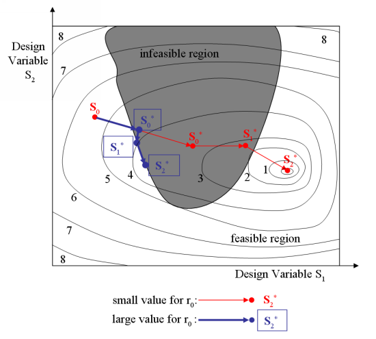
The initial value of the penalty coefficient has an impact on the behavior of
the algorithm. When  is set to a small value, a violation of the constraints does
not greatly impact the pseudo-objective function for the first iterations,
because the objective function
is set to a small value, a violation of the constraints does
not greatly impact the pseudo-objective function for the first iterations,
because the objective function  in Equation 36–5
decreases faster than the penalty term
in Equation 36–5
decreases faster than the penalty term  increases. On the contrary, when
  is set to a large value, a violation of the constraints will
dominate the pseudo-objective function, so the solution complies better with the
constraints. When the penalty coefficient is small, it is possible to cross over
a region of solutions that are infeasible due to their violation of the
constraints, and eventually reach an optimum solution in a feasible region
(where the constraints are satisfied). Whereas with a large penalty coefficient
value, it is impossible to penetrate deeply or cross over an infeasible region.
Figure 36.1: The Influence of the Initial Value of the Penalty Coefficient illustrates both
situations. The thin, red line corresponds to a case where the initial penalty
coefficient is small. For the first iteration, the solution is located deep in
the infeasible region, and during the next iteration the solution crosses over
the infeasible region. Eventually the final solution corresponds to the global
optimum. The thick, blue line corresponds to a larger value for initial penalty
coefficient. For the first iteration, the solution is located close to the
boundary of the infeasible region. During the next iteration the solution goes
back on the same side as the initial solution, and eventually reaches a final
solution at a local minimum.
is set to a large value, a violation of the constraints will
dominate the pseudo-objective function, so the solution complies better with the
constraints. When the penalty coefficient is small, it is possible to cross over
a region of solutions that are infeasible due to their violation of the
constraints, and eventually reach an optimum solution in a feasible region
(where the constraints are satisfied). Whereas with a large penalty coefficient
value, it is impossible to penetrate deeply or cross over an infeasible region.
Figure 36.1: The Influence of the Initial Value of the Penalty Coefficient illustrates both
situations. The thin, red line corresponds to a case where the initial penalty
coefficient is small. For the first iteration, the solution is located deep in
the infeasible region, and during the next iteration the solution crosses over
the infeasible region. Eventually the final solution corresponds to the global
optimum. The thick, blue line corresponds to a larger value for initial penalty
coefficient. For the first iteration, the solution is located close to the
boundary of the infeasible region. During the next iteration the solution goes
back on the same side as the initial solution, and eventually reaches a final
solution at a local minimum.
There are two criteria used to check the convergence of the method. The first is related to the objective function:
 | (36–11) |
The second criterion is related to the convergence of the constraints, as shown in the following equations:
 | (36–12) |
and
 | (36–13) |
The default value for  is 10-5.
Note that there is a difference between the convergence and the satisfaction of the constraints. The criteria expressed in Equation 36–12 and Equation 36–13 are measuring convergence, that is, whether the value of the constraint function has been dramatically reduced. On the other hand, the constraint criteria shown in Equation 36–2 and Equation 36–3 are related to the satisfaction of the constraint. Therefore, it is possible to have a converged constraint that is not well satisfied.
In the second step of the algorithm for the ALM method, the function
 is minimized to get
  using the Fletcher-Reeves (FR) method. The FR method belongs
to the conjugate gradient methods to minimize the function
using the Fletcher-Reeves (FR) method. The FR method belongs
to the conjugate gradient methods to minimize the function  without constraints. In Ansys Polyflow,
  .
.
The FR method involves multiple iterations. During an iteration, the intent is
to find a minimum along a given direction in which the function  is decreasing. At the end of the iteration, a new direction is
calculated for the next iteration. This process is repeated until convergence is
reached.
is decreasing. At the end of the iteration, a new direction is
calculated for the next iteration. This process is repeated until convergence is
reached.
The algorithm for the FR method is as follows:
With the iteration index of the FR method (
 ) set to 0 and a starting point
  equal to
  , define a tolerance
  . Also, calculate an initial direction
  , where
  is the column vector of gradients of the objective
function:
is the column vector of gradients of the objective
function: 
(36–14)
Using the direction
 , find the new point
  using the following equation:
(36–15)
where the coefficient
 is found using the line search method.
 Calculate the new conjugate gradient direction
 , according to:
(36–16)
where

(36–17)
and
 is the gradient of the objective function at a new
point:
is the gradient of the objective function at a new
point: 
(36–18)
Check for convergence. If convergence is reached, then the FR method is stopped and
 is set to
  for iteration
  of the ALM method. Otherwise, set
  and return to step 2 of the FR method.
The convergence criterion for the FR method is the following:
 | (36–19) |
with
 | (36–20) |
The direction is not always updated using Equation 36–16. Sometimes,  is reset to
 | (36–21) |
There are two cases when Equation 36–21 is used:
The efficiency of Equation 36–16 and Equation 36–17 is less and less interesting as the number of iterations of the FR method increases. Hence, a maximum number of iterations is specified, and when the simulation reaches this point the direction is set to be equal to the opposite of the gradient.
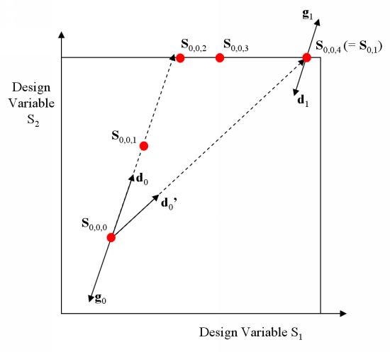
When a design variable reaches its limit, it is possible that the line search method will "move" the points along this limit. Such a situation is illustrated in Figure 36.2: Resetting the Direction to the Opposite of the Gradient with the points
 , where
  is the iteration index of the line search. Because the
points
is the iteration index of the line search. Because the
points  ,
,  , and
, and  are located along the limit of design variable
 , the initial direction
  and the direction
  between the initial and the final points of the line
search are not the same. In such circumstances, the direction is reset
to the opposite of the gradient.
between the initial and the final points of the line
search are not the same. In such circumstances, the direction is reset
to the opposite of the gradient.
In the second step of the algorithm for the FR method, it is necessary to find
a value for the coefficient  that minimizes
  . In order to do this, the line search (LS) method performs
several calculations of
. In order to do this, the line search (LS) method performs
several calculations of  , during which the target value
  is varied. Note that the subscript
  refers to the iteration index of the LS method, whereas the
subscripts
refers to the iteration index of the LS method, whereas the
subscripts  and
and  refer to the iteration indices of the ALM and FR method,
respectively.
refer to the iteration indices of the ALM and FR method,
respectively.
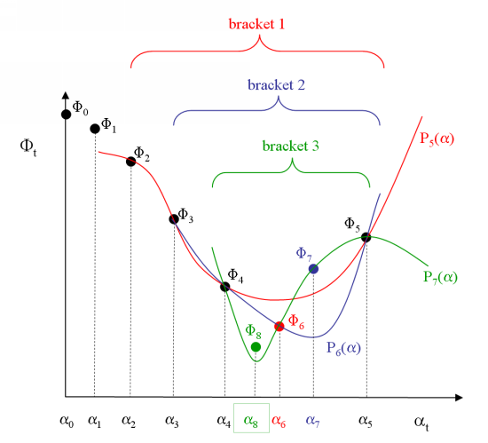
Figure 36.3: An Example of the LS Algorithm illustrates an example of
the LS method algorithm. Starting with  , an initial value
  is calculated. The slope of the function at this point is
negative, as the direction
is calculated. The slope of the function at this point is
negative, as the direction  was specifically defined to follow a decreasing gradient. A
target value
was specifically defined to follow a decreasing gradient. A
target value  is then used to calculate
  . The initial target value
  is based upon the distance of the current point from the
bounds of the design variable, the value and the slope of the function
is based upon the distance of the current point from the
bounds of the design variable, the value and the slope of the function
 , and sometimes the value of
  (the coefficient of the previous FR method iteration). As
shown in Figure 36.3: An Example of the LS Algorithm,
(the coefficient of the previous FR method iteration). As
shown in Figure 36.3: An Example of the LS Algorithm,  is smaller than
  , so
, so  is increased to the new target value
  , and
, and  is calculated. This process is repeated to generate the
successive target values
is calculated. This process is repeated to generate the
successive target values  ,
,  , and
, and  . The process is interrupted when
  (that is, when
  ). At this point, the minimum is assumed to be located
somewhere between
). At this point, the minimum is assumed to be located
somewhere between  and
and  . As a first attempt at finding it, a new target value
 is generated that minimizes
  .
.  is an interpolation of the target values in bracket 1, and can
be expressed thusly:
is an interpolation of the target values in bracket 1, and can
be expressed thusly:
 | (36–22) |
Having found  , it is then possible to calculate
  . In a similar fashion, the target values in bracket 2 are used
to calculate
. In a similar fashion, the target values in bracket 2 are used
to calculate  ,
,  , and
, and  , and the target values in bracket 3 are used to calculate
 ,
,  , and
, and  . The line search ends at this point because convergence is
reached.
. The line search ends at this point because convergence is
reached.
The general algorithm for the LS method can be stated as follows:
With the iteration index of the LS method (
 ) equal to 0, set
  and calculate
  using the following relation:
(36–23)
where
 and
and  are the current iteration indices of the ALM and FR
methods, respectively.
are the current iteration indices of the ALM and FR
methods, respectively. Set
 and generate a value for
  such that
  . Then calculate
  using Equation 36–23.
 If
 , return to step 2. Otherwise, proceed to step 4.
Generate a function
 that interpolates the last four values of
 (use less values if
  ). Then set
  and set
  equal to the minimum value of
  .
. Calculate
 using Equation 36–23.
 Check for convergence. If convergence is reached, then the LS method is stopped and
 is set to
  for iteration
  of the FR method. Otherwise, return to step 4 of the
LS method.
of the FR method. Otherwise, return to step 4 of the
LS method.
The process is deemed to be converged if the number of iterations has reached
a predefined "maximum number of iterations to reach minimum", if  , or if two successive solutions are very close.
The LS method algorithm is CPU intensive, because it corresponds to the
computation of the flow solution. For this reason, it is more efficient to
perform a small number of iterations (with a resulting accuracy that is lower)
for the LS method. Hence, the default value for "the maximum number of
iterations to reach minimum" is  , where
  is the iteration number at the beginning of step 4 of the LS
method algorithm.
is the iteration number at the beginning of step 4 of the LS
method algorithm.
If the flow problem is governed by nonlinear equations, the LS method can fail
when trying to calculate  . Under such circumstances, the value of
  is reduced and subiterations are used to reach a target value,
resulting in intermediate values of the function
is reduced and subiterations are used to reach a target value,
resulting in intermediate values of the function  . If a target value cannot be reached, the last successful
intermediate value is assumed as the target value, and the LS method continues.
. If a target value cannot be reached, the last successful
intermediate value is assumed as the target value, and the LS method continues.
When it becomes necessary to calculate intermediate values of  , the LS method proceeds to find a minimum
  that is based on the target values only. A comparison is then
made to see if any of the intermediate values of
that is based on the target values only. A comparison is then
made to see if any of the intermediate values of  are smaller than
  ; if this is the case, then the associated intermediate value
of
; if this is the case, then the associated intermediate value
of  is taken as the solution of the LS method.