These sections describe the oSP3D workflow:
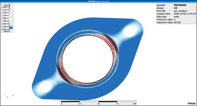
Running a DOE with Ansys optiSLang obtains 45 designs, each consisting of a set of scalar input parameters, the contact pressure field, and contact state field.
The following image shows the simulated contact pressure field for design 4.
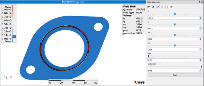
Using the imported scalar input parameters and field designs as training data, two field-MOPs are created within seconds.
This image shows the field-MOP with the contact state field as the output:
This next image shows the field-MOP with the contact pressure field as the output:
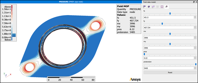
Note: Using the sliders to change the scalar input parameters provides instant results.
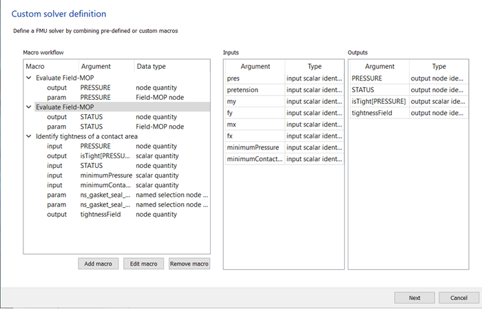
A custom solver is created and exported to an FMU2.0 file.
oSP3D allows you to interactively combine the three analysis steps:
Evaluate the contact pressure field-MOP.
Evaluate the contact state field-MOP.
Run the algorithm for identifying tightness.
oSP3D tracks input and output parameters. This image shows the definition for the custom solver: