


Another topology optimization technology method is the level-set based method. Originally used for computational fluid dynamics (CFD) to track fluid-interface it is also applied in structural optimization.
Shape Description
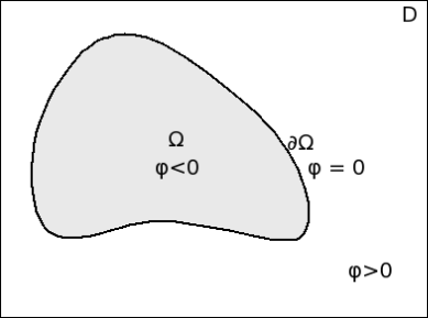
This method manages shape description through pure geometric information and defines a shape without ambiguity. That is, for the shape, defined over the working domain, using an auxiliary function, denoted as the level-set function, specifies positive, zero, or negative values, such that:
|
|
|

Note:
This implicit representation of the shape enables you to make topological changes without needing to detect topological modifications and reconstruct shape parametrizations.
Provides a convenient framework for the calculation of geometric quantities, such as the exterior normal vector:
 .
.For the level-set functions that provide the same shape description, Ansys uses the signed-distance function (SDF) [DF2012], defined as:

where
 denotes the standard Euclidian distance from a point
 to the boundary
  .
. The level-set function is discretized at vertices of the mesh and interpolated inside the elements.
Shape Evaluation
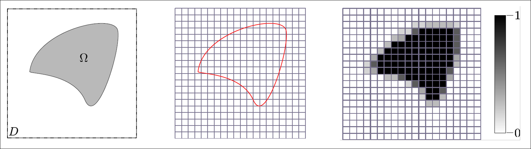
The application evaluates the criteria on a fixed mesh. However, the definition of the mechanical properties is simple and generic, that is:
Any element lying inside of the shape has a density value of 1.
Any element lying outside the shape is specified as a void-material.
As to the one layer of elements cut by the zero level-set, they receive an intermediate density in accordance with the solid fraction.
|
|
|
Pseudo-density used for the modification of the mechanical properties. |
Using the ersatz-material approach [5], each material property is interpolated as  , where Evoid <<
Esolid corresponds to the material
properties of a weak material representing the void.
, where Evoid <<
Esolid corresponds to the material
properties of a weak material representing the void.
Shape Derivative
The application computes the shape derivative using the continuous formalism
defined by Hadamard (see [5]).
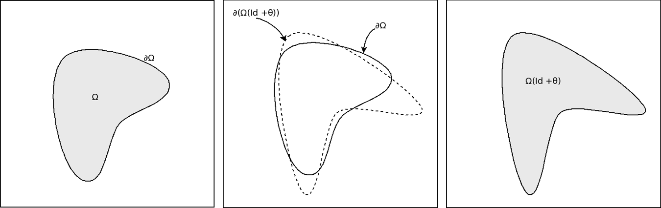
That is, given a shape perturbation  , the asymptotic expansion reads:

Where:
 is current shape. is current shape. |
 is the shape perturbation. is the shape perturbation. |
 is the new shape. is the new shape. |
The shape derivative usually admits the following form:

For the form, the integrand,  , depends on the criterion,
  , through both the solution state of the mechanical problem and
some corresponding adjoint-state.
, through both the solution state of the mechanical problem and
some corresponding adjoint-state.
|
|
|
Shape perturbation by a vector field |

Shape Update
Given a shape perturbation  , the application updates the shape by solving a transport equation
for the level-set function [BDF2012]:
, the application updates the shape by solving a transport equation
for the level-set function [BDF2012]:

Summary
The degrees of freedom for this method are based on the boundary of the shape.
- Strengths
Enables you to easily manage topological changes. It delivers an unambiguous solution. - Place in Design Stage
Used early in the design process to sketch conceptual designs.
- Limitations
Produces a less accurate evaluation that the body-fitted approach. Due to the heavy machinery, the run is sometimes more expensive compared to the density method. - Tips
Use a uniform mesh to equally capture geometric details for the entire domain.
References
[4] C. Dapogny, P. Frey, Computation of the signed distance function to a discrete contour on adapted triangulation, Calcolo, 2012.
[5] G. Allaire, F. Jouve, AM Toader, Structural optimization using sensitivity analysis and a level-set method, Journal of computational physics, 2004.
[6] C. Bui, C. Dapogny, P. Frey. An accurate anisotropic adaptation method for solving the level set advection equation, International Journal for Numerical Methods in Fluids, 2012.
[7] S. Osher, JA Sethian, Fronts propagating with curvature-dependent speed: Algorithms based on Hamilton-Jacobi formulations, Journal of computational physics, 1988.