


The density-based method belongs to the family of topology optimization technology. Adopting the logic of immersed boundary methods, this method aims to optimize the distribution of material within a working domain by varying a density field ranging from 0 to 1. Topology optimization technology, which first appeared in the framework of the homogenization method for composites [1] [3]. Simplified approaches, such as Solid Isotropic Material with Penalization method (SIMP), followed and were devised to force the density to approach either 0 or 1, making them applicable for standard solid structures.
Shape Description
You can characterize the density-based approach as a large-scale parametric optimization where the DOF is the “density.” That is, a unit-less variable ranging from 0 to 1, where:
A value of zero (0) virtually removes elements to create virtual voids.
A value of one (1) specifies an element with a material.
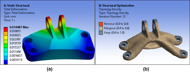
As a result, this method does not deliver a shape but an optimized density-field. To create an unambiguous design, the application forces the density to approach 0 or 1 and then removes any intermediate densities. Here is an example of a part defined with a density-threshold of 0.5 (default).
Where:
(a) is the optimal distribution of density (over the working domain).
(b) is the resulting shape (while drawing the iso-surface corresponding to 0.5 – density)
Shape Evaluation
For shape evaluation using the density-field,  , it is critical to properly update the material properties.
Specifically, the application updates:
, it is critical to properly update the material properties.
Specifically, the application updates:
Young modulus and mass for static structural and modal analyses.
Conductivity and mass for thermal analyses.
To force solutions to approach either zero (0) or one (1), Ansys uses the following widely documented interpolation schemes:
 (linear interpolation for the mass).
 (power-law interpolation for stiffness [BS2003]).
Note: For the above calculations, Mvoid << Msolid and Kvoid << Ksolid correspond to the material properties of a weak material representing the void.
Shape Derivative
The shape derivative used in gradient-based optimizers for the density-based method is calculated from the derivative with respect to the density. Furthermore, for:
Geometric criteria, the computation is analytical.
Physics-based criteria, the adjoint approach is used.
Shape Update
By adding the descent direction  , derived from the gradient-based optimizer, to the current density
field
, derived from the gradient-based optimizer, to the current density
field  , the application computes a new density field
  . The calculation is represented as:

representing the new shape:  .
.
Summary
Degrees of freedom for this method are based on the density of the elements or the density at the nodes.
- Strengths
Enables you to easily manage topological changes. It is based on the development of light machinery and enables fast convergence. - Place in Design Stage
Used early in the design process to sketch designs.
- Limitations
Can sometimes deliver an ambiguous solution, including intermediate densities that do not provide the most ideal optimized part. Produces a less accurate evaluation than the body-fitted approach. - Tips
Use a uniform mesh to equally capture geometric details for the entire domain.
References
[1] MP Bendsoe, N. Kikuchi, Generating optimal topologies in structural design using a homogenization method, Computer methods in applied mechanics and engineering, 1988.
[2] MP Bendsoe, O. Sigmund, Topology optimization: theory, methods, and applications, Springer Science & Business Media, 2003.
[3] F. Murat, L. Tartar, Calcul des Variations et Homogeneisation, In Les Methodes de l Homogeneisation Theorie et Applications en Physique, Coll. Dir. Etudes et Recherches EDF, 57, Eyrolles, Paris, pp.319-369, 1985.