VM-LSDYNA-FLUID-001
VM-LSDYNA-FLUID-001
Blasius Solution
Overview
| Reference: |
Blasius, H. (1908). Grenzschichten in gliissigkeiten mit kleiner reibung. Zeitschrift fiir Mthematik und Physik, 56(1), 1-37. Caldichoury, I. & Paz, R. (2014). Incompressible fluid solver in LS-DYNA. ICFD Theory Manual. Tested with LS-DYNA R7.0 Revision Beta. |
| Analysis Type(s): | Incompressible CFD |
| Input Files: | Link to Input Files Download Page |
Test Case
This test case reproduces a two-dimensional stationary and incompressible laminar flow over a flat plate. The purpose is to validate the drag force coefficient on the plate against the classic Blasius solution (1908).
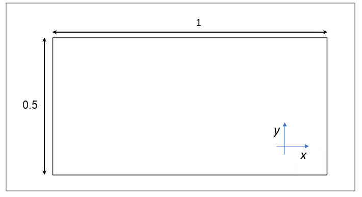
The domain consists of a rectangular box with an inflow of prescribed velocity and an outflow of prescribed pressure. Also, the lower and upper sides of the boundary have non-slip and free-slip conditions, respectively. The domain size and relevant quantities are shown in the problem sketch below.
For this test case, all units of measure are consistent (length = m, time = s, mass = kg, force = N, pressure = Pa).
| Material Properties | Geometric Properties | Loading |
|---|---|---|
|
Fluid: • Flow density ρ = 1 • Flow kinematic viscosity μ = 104 |
Mesh size: • Fluid plate boundaries elements length : 0.01 • Anisotropic elements added to Boundary Layer: 5
Geometry: • Plate length L = 1 • Inlet and outlet height H = 0.5 |
Fluid: • Inflow speed V = 1 • Outflow pressure p = 0 |
Analysis Assumptions and Modeling Notes
The behavior of the flow is characterized by the Reynolds number:
 | (3) |
where ρ is the fluid's density, L is the characteristic length of the problem (the plate length), V is the inlet velocity, and μ is the dynamic viscosity of the flow.
It can be demonstrated that for Re < 105, the flow is laminar. For 105 < Re < 106, the flow experiences a laminar-to-turbulent transition.
For this test, a combination of physical parameters is chosen for which Re = 104. The resulting frictional drag force will be compared to the result proposed by Blasius:
 | (4) |
It should be noted that for 2D problems nondimensional coefficients are evaluated using the following relation:
 | (5) |
where Fxx is the relative dimensional force.
In order to negate the influence of the outer boundaries, the height of the domain H will be ten times larger than the boundary layer δ, which can be estimated using the following formula from the reference:
 | (6) |
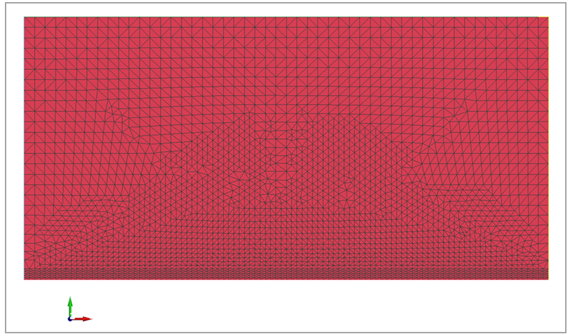
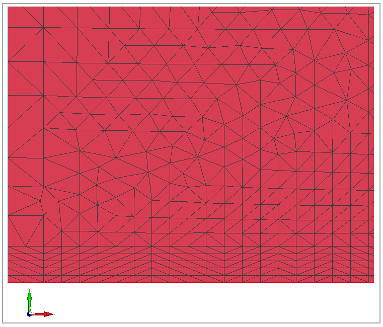
The boundary layer over the flat plate is modeled using five rectangular elements. A picture of the domain's mesh is shown in Figure 123, while Figure 124 shows a detail of the mesh refinement for the boundary layer.
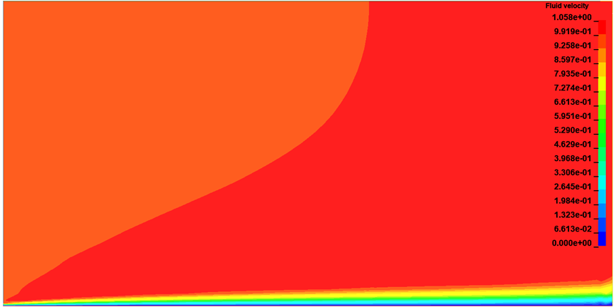
Results Comparison
The resulting fluid velocity can be observed in Figure 125. As expected, a parabolic flow develops close to the solid boundary layer. For the numerical drag calculation, the ICFD solver does not include the first and last elements of the plate. For this reason, in this scenario, it is necessary to modify the analytical friction drag coefficient to 0.01328. The solver is in close agreement, calculating the numerical friction drag coefficient to be 0.01344, an error of approximately 1.2%.