VM-LSDYNA-EMAG-011

VM-LSDYNA-EMAG-011
Long Cylinder in a Uniform Sinusoidal Field (TEAM 2)

Overview

Reference:	Ida, N. (1998). Infinite cylinder in a uniform sinusoidal field (comparison of results, problem 2). COMPEL - The International Journal for Computation and Mathematics in Electrical and Electronic Engineering, 7, 29-45.
Analysis Type(s):	Electromagnetism
Element Type(s):	Solid Elements ELFORM 1
Input Files:	Link to Input Files Download Page

Test Case

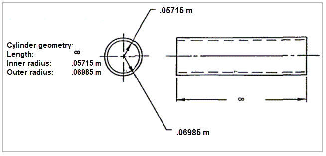
The TEAM 2 problem consists of an infinitely long cylinder, where a uniform field of 0.1 Tesla at 60 Hz is applied perpendicular to its axis. The cylinder is made of aluminum alloy 6061. The properties and loading are depicted below.

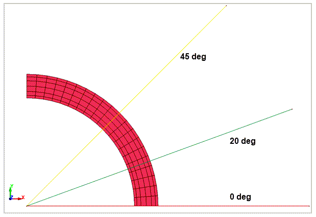
The objective of the test is to measure the amplitude and phase of the magnetic field along the Y axis. Points along three lines from (R = 0,Z = 0) to (R = 0.15,Z = 0) at 0 degrees, 20 degrees and 45 degrees are created, so that the magnetic field along these lines can be extracted and compared with the analytical solution. In addition, the total power loss and forces on the X and Y axes on one quarter of the cylinder are calculated.

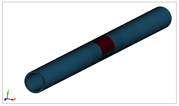
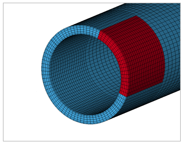
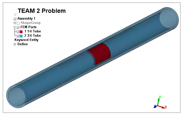
Figure 221: Problem sketch and dimensions

The LS-DYNA model is not infinite but has a total length of two meters. The red section of the mesh is differentiated and finer to extract the power loss and the forces. The lines to extract the magnetic field are also shown below in Figure 223.

Figure 222: Problem setup

Figure 223: Location of the lines to extract the magnetic field

Material Properties	Geometric Properties	Loading

Analysis Assumptions and Modeling Notes

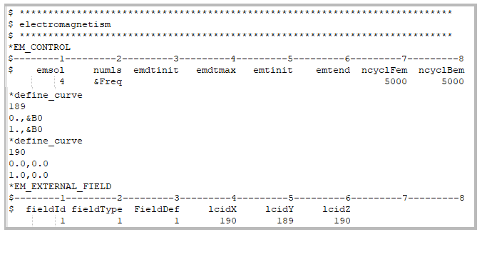
LS-DYNA *EM_CONTROL card is set to 4 to activate the Frequency-Based Eddy Current solver. The current is applied using *EM_EXTERNAL_FIELD pointing to a load curve, where the magnetic field along time is specified. In this case, since the magnetic field is constant, the curve is flat (values represented by the &B0 variable).

The mesh is formed by solid elements formulation 1, which is a constant stress solid element. The thickness of the cylinder is represented by six elements. The red part of the mesh is finer along the cylinder's axis to better capture some of the results.

Figure 224: Cut section of the mesh.

Red mesh is finer than the surroundings to better capture the results.

Results Comparison

The experimental results are compared with LS-DYNA output. Magnetic field results are extracted from em_pointout.dat for magnitude and em_pointout_phi.dat for phase.

Figure 225: Magnetic field amplitude comparison between simulation and experiment at 0 degrees

Figure 226: Magnetic field phase comparison between simulation and experiment at 0 degrees

Figure 227: Magnetic field phase comparison between simulation and experiment at 20 degrees

Figure 228: Magnetic field amplitude comparison between simulation and experiment at 45 degrees

Figure 229: Magnetic field Phase comparison between simulation and experiment at 45 degrees

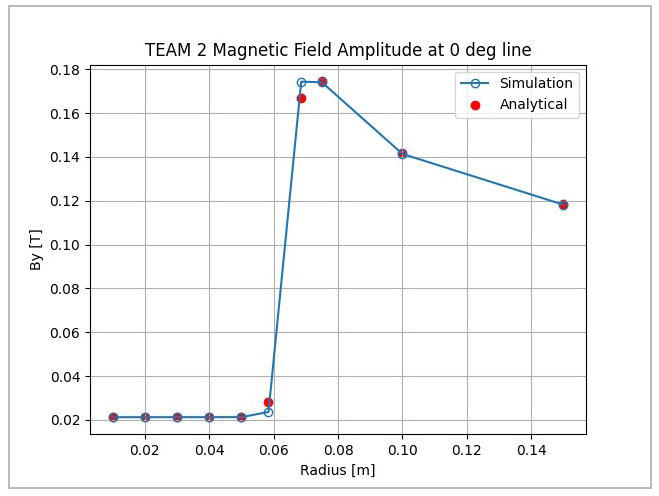
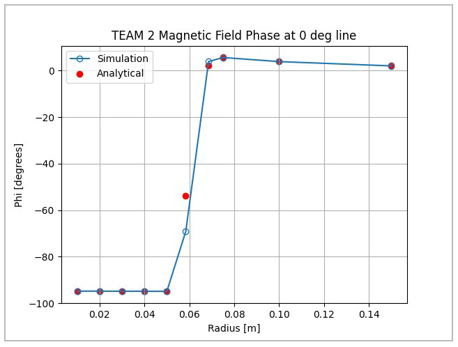
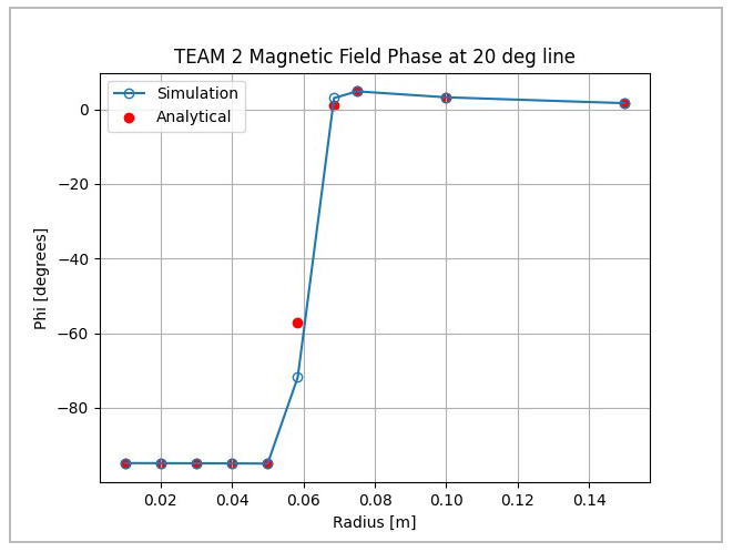
The error between the analytical results and the simulation is presented in Table 27 through Table 32. There is a high level or correlation between the analytical solution and the solver. The largest discrepancies are for those points very close to and inside the cylinder.

Table 27: Amplitude y-Bfield at several cylinder radiuses for 0 degree line

Result	Target (T)	Workbench LS-DYNA (T)	Error (%)
y-Bfield (phase) at R = 0.01 m	0.0211	0.0212	0.47
y-Bfield (phase) at R = 0.02 m	0.0211	0.0212	0.48
y-Bfield (phase) at R = 0.03 m	0.0211	0.0212	0.50
y-Bfield (phase) at R = 0.04 m	0.0211	0.0212	0.52
y-Bfield (phase) at R = 0.05 m	0.0211	0.0212	0.56
y-Bfield (phase) at R = 0.05842 m	0.028	0.0236	15.79
y-Bfield (phase) at R = 0.06858 m	0.1667	0.1744	4.60
y-Bfield (phase) at R = 0.075 m	0.1745	0.1741	0.23
y-Bfield (phase) at R = 0.1 m	0.1418	0.1414	0.28
y-Bfield (phase) at R = 0.15 m	0.1185	0.1182	0.25

Table 28: Phase y-Bfield at several cylinder radiuses for 0 degree line

Result	Target (T)	Workbench LS-DYNA (T)	Error (%)
y-Bfield (phase) at R = 0.01 m	-95	-94.827	0.18
y-Bfield (phase) at R = 0.02 m	-95	-94.840	0.17
y-Bfield (phase) at R = 0.03 m	-95	-94.860	0.15
y-Bfield (phase) at R = 0.04 m	-95	-94.889	0.12
y-Bfield (phase) at R = 0.05 m	-95	-94.925	0.08
y-Bfield (phase) at R = 0.05842 m	-53.8	-69.143	<20
y-Bfield (phase) at R = 0.06858 m	2.1	3.922	<20
y-Bfield (phase) at R = 0.075 m	5.7	5.652	0.84
y-Bfield (phase) at R = 0.1 m	3.9	3.897	0.08
y-Bfield (phase) at R = 0.15 m	2.1	2.054	2.17

Table 29: Amplitude y-Bfield at several cylinder radiuses for 20 degree line

Result	Target (T)	Workbench LS-DYNA (T)	Error (%)
y-Bfield (phase) at R = 0.01 m	0.0211	0.0212	0.47
y-Bfield (phase) at R = 0.02 m	0.0211	0.0212	0.48
y-Bfield (phase) at R = 0.03 m	0.0211	0.0212	0.51
y-Bfield (phase) at R = 0.04 m	0.0211	0.0212	0.54
y-Bfield (phase) at R = 0.05 m	0.0211	0.0212	0.58
y-Bfield (phase) at R = 0.05842 m	0.027	0.0231	14.53
y-Bfield (phase) at R = 0.06858 m	0.1485	0.1552	4.48
y-Bfield (phase) at R = 0.075 m	0.157	0.1566	0.27
y-Bfield (phase) at R = 0.1 m	0.1319	0.1316	0.22
y-Bfield (phase) at R = 0.15 m	0.1142	0.1139	0.28

Table 30: Phase y-Bfield at several cylinder radiuses for 20 degree line

Result	Target (T)	Workbench LS-DYNA (T)	Error (%)
y-Bfield (phase) at R = 0.01 m	-95	-94.83	0.18
y-Bfield (phase) at R = 0.02 m	-95	-94.84	0.16
y-Bfield (phase) at R = 0.03 m	-95	-94.87	0.14
y-Bfield (phase) at R = 0.04 m	-95	-94.90	0.10
y-Bfield (phase) at R = 0.05 m	-95	-94.95	0.05
y-Bfield (phase) at R = 0.05842 m	-57.3	-71.85	<20
y-Bfield (phase) at R = 0.06858 m	1.2	3.00	<20
y-Bfield (phase) at R = 0.075 m	4.8	4.80	0.08
y-Bfield (phase) at R = 0.1 m	3.2	3.20	0.03
y-Bfield (phase) at R = 0.15 m	1.7	1.63	4.29

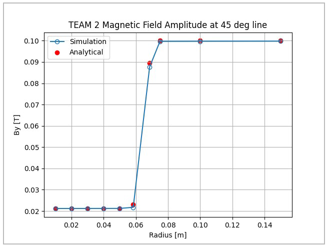
Table 31: Amplitude y-Bfield at several cylinder radiuses for 45 degree line

Result	Target (T)	Workbench LS-DYNA (T)	Error (%)
y-Bfield (phase) at R = 0.01 m	0.0211	0.0212	0.47
y-Bfield (phase) at R = 0.02 m	0.0211	0.0212	0.49
y-Bfield (phase) at R = 0.03 m	0.0211	0.0212	0.53
y-Bfield (phase) at R = 0.04 m	0.0211	0.0212	0.58
y-Bfield (phase) at R = 0.05 m	0.0211	0.0212	0.64
y-Bfield (phase) at R = 0.05842 m	0.023	0.0218	5.43
y-Bfield (phase) at R = 0.06858 m	0.0896	0.0876	2.19
y-Bfield (phase) at R = 0.075 m	0.1	0.0997	0.31
y-Bfield (phase) at R = 0.1 m	0.1	0.0997	0.27
y-Bfield (phase) at R = 0.15 m	0.1	0.0998	0.23

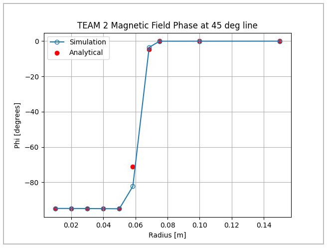
Table 32: Phase y-Bfield (T) at several cylinder radiuses for 45 degree line

Result	Target (T)	Workbench LS-DYNA (T)	Error (%)
y-Bfield (phase) at R = 0.01 m	-95	-94.83	0.18
y-Bfield (phase) at R = 0.02 m	-95	-94.86	0.15
y-Bfield (phase) at R = 0.03 m	-95	-94.90	0.11
y-Bfield (phase) at R = 0.04 m	-95	-94.95	0.05
y-Bfield (phase) at R = 0.05 m	-95	-95.03	0.03
y-Bfield (phase) at R = 0.05842 m	-71.2	-82.31	15.60
y-Bfield (phase) at R = 0.06858 m	-4.6	-3.55	<20
y-Bfield (phase) at R = 0.075 m	0	-0.05	5.01
y-Bfield (phase) at R = 0.1 m	0	-0.04	4.15
y-Bfield (phase) at R = 0.15 m	0	-0.03	3.06

The results for the total power loss and forces in one quarter of the cylinder are obtained from the em_partDataFreq_0001.dat file which contains the results for the highlighted volume in Figure 230. Since this volume represents one tenth of the total length, the results must be multiplied by this amount to account for the overall one-quarter of the cylinder. In addition, the total length of the cylinder is two meters. As the reference result is given per meter of length, the simulation results must be divided by two. Using this information, the results are derived:

(35)

(36)

(37)

Figure 230: Cylinder volume used to extract power loss and forces

A strong correlation between the analytical result and the simulation is evident in Table 33.

Table 33: Total Power Loss (W/m) and Forces (N/m) for one quarter of the cylinder

Result	Target	Workbench LS-DYNA	Error (%)
Total Power Loss (W/m)	2288.2	2260.29	1.22
Fx (N/m)	-333.4	-370.73	11.20
Fy (N/m)	-166.7	-143.88	13.69