


VM-LSDYNA-EMAG-010
VM-LSDYNA-EMAG-010
Asymmetrical Conductor with a Hole (TEAM 7)
Overview
| Reference: | Fujiwara, K. & Nakata, T. (1990). Results for benchmark problem 7 (Asymmetrical Conductor with a Hole). COMPEL - The International Journal for Computation and Mathematics in Electrical and Electronic Engineering, 9(3), 137-154. |
| Analysis Type(s): | Electromagnetism |
| Element Type(s): | Solid Elements ELFORM 1 |
| Input Files: | Link to Input Files Download Page |
Test Case
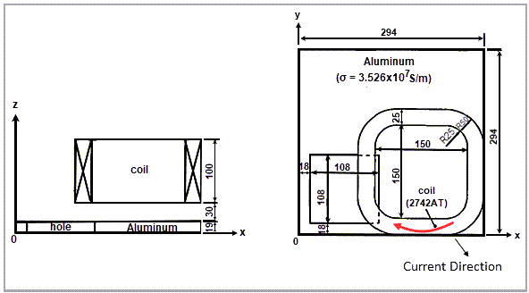
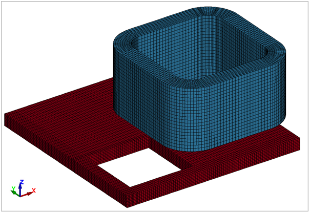
This TEAM 7 problem consists of a thick aluminum plate with a hole which is placed eccentrically and set unsymmetrically in a non-uniform magnetic field. The field is produced by the exciting current which varies sinusoidally with time. The Frequency Eddy Current solver is used to retrieve the real and imaginary parts of the magnetic flux between the coil and plate. Results are compared with the reference.
The conductivity of the plate is 3.526×10⁷ S/m. The current is set to 2742 AT (Ampere-Turn). The results are extracted for two different frequencies, 50 Hz and 200 Hz. Each is a separate set of tests.
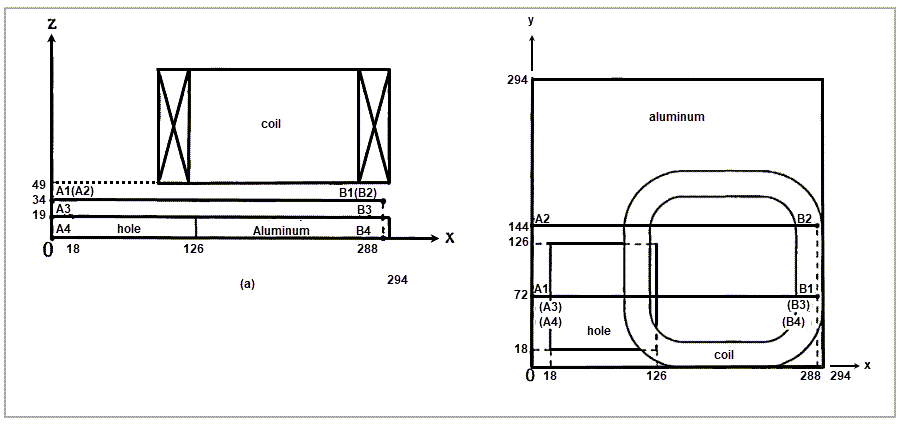
The magnetic field is obtained along the two lines between the plate and the coil. These lines are defined as A1B1 and A2B2 lines. Both lines are located at the same Z coordinate and different Y coordinates as shown in Figure 217.
Analysis Assumptions and Modeling Notes
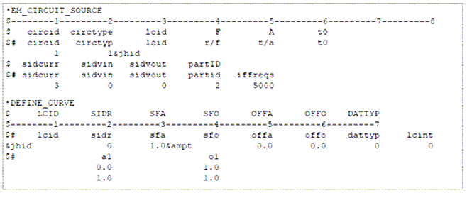
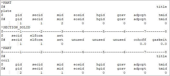
LS-DYNA *EM_CONTROL card is set to 4 to activate the Frequency-based Eddy Current solver. The current is applied using *EM_CIRCUIT_SOURCE card, which points to a *DEFINE_CURVE card containing the ampere-turns. The variable jhid is the load case ID.
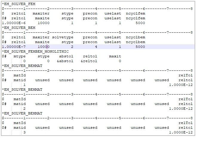
The monolithic solver is used.
The mesh is formed by a solid mesh with element formulation 1 which is a constant stress solid element. Two parts are defined, one for the coil and one for the plate.
Results Comparison
The analytic solution is compared with LS-DYNA output. Simulation results are extracted from the em_pointout.dat and em_pointout_phi.dat files. The first file provides the magnitude, and the second one provides the phase. To calculate the real and imaginary part and compare it with the experimental data, the following formulas are applied:
 | (33) |
 | (34) |
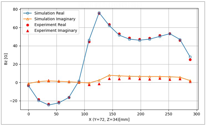
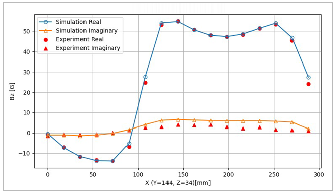
The results for line A1B1 and A2B2 are shown for 50 Hz.
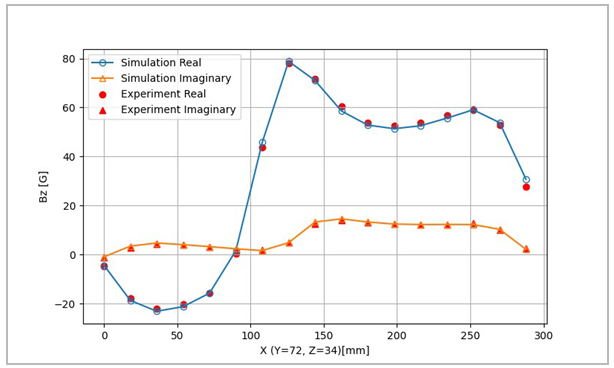
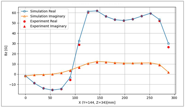
The error between the experiment and the simulation is presented in the tables below. There are a couple of points with a relative error above 10% and one above 20% at x = 90 mm. Nevertheless, the quantities are small and the differences compared to the values are low. Furthermore, it is possible that the reference values vary slightly from one measurement to another, especially at a location where a slight variation may increase or decrease the measured magnetic field. Overall, results are in accordance with the reference.
Table 19: z-Bfield (real, in G) for several x coordinates (y=72 mm, z=34 mm) for 50 Hz at line A1B1
| Result | Target (G) |
Workbench
LS-DYNA
(G) | Error (%) |
|---|---|---|---|
| zBfield real at x = 0 mm | -3.63 | -3.40 | 6.29 |
| zBfield real at x = 18 mm | -18.46 | -19.62 | 6.30 |
| zBfield real at x = 36 mm | -23.62 | -24.66 | 4.40 |
| zBfield real at x = 54 mm | -21.59 | -22.39 | 3.69 |
| zBfield real at x = 72 mm | -16.09 | -16.45 | 2.27 |
| zBfield real at x = 90 mm | 0.23 | 1.47 | >20 |
| zBfield real at x = 108 mm | 44.35 | 46.15 | 4.06 |
| zBfield real at x = 126 mm | 75.53 | 76.16 | 0.83 |
| zBfield real at x = 144 mm | 63.42 | 62.18 | 1.96 |
| zBfield real at x = 162 mm | 53.20 | 51.57 | 3.06 |
| zBfield real at x = 180 mm | 48.66 | 47.29 | 2.83 |
| zBfield real at x = 198 mm | 47.31 | 46.12 | 2.51 |
| zBfield real at x = 216 mm | 48.31 | 47.26 | 2.17 |
| zBfield real at x = 234 mm | 51.26 | 50.25 | 1.97 |
| zBfield real at x = 252 mm | 53.61 | 53.23 | 0.71 |
| zBfield real at x = 270 mm | 46.11 | 46.99 | 1.90 |
| zBfield real at x = 288 mm | 24.96 | 28.09 | 12.53 |
Table 20: . z-Bfield (imaginary, in G) for several x coordinates (y=72 mm, z=34 mm) for 50 Hz at line A1B1
| Result | Target (G) |
Workbench
LS-DYNA
(G) | Error (%) |
|---|---|---|---|
| zBfield imaginary at x = 0 mm | -1.16 | -0.95 | 18.20 |
| zBfield imaginary at x = 18 mm | 2.84 | 3.43 | 20.89 |
| zBfield imaginary at x = 36 mm | 4.15 | 4.70 | 13.37 |
| zBfield imaginary at x = 54 mm | 4.00 | 4.04 | 1.08 |
| zBfield imaginary at x = 72 mm | 3.07 | 3.23 | 5.32 |
| zBfield imaginary at x = 90 mm | 2.31 | 2.34 | 1.37 |
| zBfield imaginary at x = 108 mm | 1.89 | 1.60 | 15.19 |
| zBfield imaginary at x = 126 mm | 4.97 | 4.82 | 2.94 |
| zBfield imaginary at x = 144 mm | 12.61 | 13.26 | 5.15 |
| zBfield imaginary at x = 162 mm | 14.15 | 14.57 | 2.98 |
| zBfield imaginary at x = 180 mm | 13.04 | 13.28 | 1.81 |
| zBfield imaginary at x = 198 mm | 12.40 | 12.45 | 0.42 |
| zBfield imaginary at x = 216 mm | 12.05 | 12.22 | 1.39 |
| zBfield imaginary at x = 234 mm | 12.27 | 12.27 | 0.03 |
| zBfield imaginary at x = 252 mm | 12.66 | 12.22 | 3.44 |
| zBfield imaginary at x = 270 mm | 9.96 | 10.30 | 3.45 |
| zBfield imaginary at x = 288 mm | 2.36 | 2.11 | 10.74 |
Table 21: z-Bfield (real, in G) for several x coordinates (y=144 mm, z=34 mm) for 50 Hz at line A2B2
| Result | Target (G) |
Workbench
LS-DYNA
(G) | Error (%) |
|---|---|---|---|
| zBfield real at x = 0 mm | -1.83 | -1.53 | 16.65 |
| zBfield real at x = 18 mm | -8.50 | -8.78 | 3.27 |
| zBfield real at x = 36 mm | -13.60 | -13.88 | 2.03 |
| zBfield real at x = 54 mm | -15.21 | -15.52 | 2.05 |
| zBfield real at x = 72 mm | -14.48 | -14.37 | 0.73 |
| zBfield real at x = 90 mm | -5.62 | -3.29 | >20 |
| zBfield real at x = 108 mm | 28.77 | 32.55 | 13.15 |
| zBfield real at x = 126 mm | 60.34 | 61.30 | 1.59 |
| zBfield real at x = 144 mm | 61.84 | 61.82 | 0.04 |
| zBfield real at x = 162 mm | 56.64 | 56.44 | 0.35 |
| zBfield real at x = 180 mm | 53.40 | 53.21 | 0.36 |
| zBfield real at x = 198 mm | 52.36 | 52.44 | 0.15 |
| zBfield real at x = 216 mm | 53.93 | 53.73 | 0.36 |
| zBfield real at x = 234 mm | 56.82 | 56.67 | 0.26 |
| zBfield real at x = 252 mm | 59.48 | 59.51 | 0.04 |
| zBfield real at x = 270 mm | 52.08 | 53.31 | 2.36 |
| zBfield real at x = 288 mm | 26.56 | 29.97 | 12.83 |
Table 22: z-Bfield (imaginary, in G) for several x coordinates (y=144 mm, z=34 mm) for 50 Hz at line A2B2
| Result | Target (G) |
Workbench
LS-DYNA
(G) | Error (%) |
|---|---|---|---|
| zBfield imaginary at x = 0 mm | -1.63 | -1.76 | 7.93 |
| zBfield imaginary at x = 18 mm | -0.60 | -0.73 | 20.84 |
| zBfield imaginary at x = 36 mm | -0.43 | -0.40 | 5.92 |
| zBfield imaginary at x = 54 mm | 0.11 | 0.07 | 32.89 |
| zBfield imaginary at x = 72 mm | 1.26 | 1.43 | 13.20 |
| zBfield imaginary at x = 90 mm | 3.40 | 3.90 | 14.61 |
| zBfield imaginary at x = 108 mm | 6.53 | 7.20 | 10.27 |
| zBfield imaginary at x = 126 mm | 10.25 | 10.53 | 2.77 |
| zBfield imaginary at x = 144 mm | 11.83 | 12.40 | 4.82 |
| zBfield imaginary at x = 162 mm | 11.83 | 12.03 | 1.70 |
| zBfield imaginary at x = 180 mm | 11.01 | 11.21 | 1.86 |
| zBfield imaginary at x = 198 mm | 10.58 | 10.80 | 2.06 |
| zBfield imaginary at x = 216 mm | 10.80 | 10.76 | 0.36 |
| zBfield imaginary at x = 234 mm | 10.54 | 10.94 | 3.81 |
| zBfield imaginary at x = 252 mm | 10.62 | 11.04 | 4.00 |
| zBfield imaginary at x = 270 mm | 9.03 | 9.46 | 4.72 |
| zBfield imaginary at x = 288 mm | 1.79 | 1.93 | 7.66 |
The results for line A1B1 and A2B2 are shown for 200 Hz.
The error between the experiment and the simulation is presented in the tables below. For this case, the conclusions are similar to those for 50 Hz. The real part shows a better correlation between the experiment and simulation, with a lower correlation for the same points compared to 50 Hz. In the same way, the magnetic field is very low with a high gradient, which means that a slight variation in the measurement might end up with an important increase/decrease of the measured magnetic field. Regarding the imaginary part, the curve is flatter compared to 50 Hz, and closer to zero. According to the reference, when the size of the sensor is large compared to the gradient of the magnetic field, measurement error increases. This might explain the lower degree of correlation between the experiment and the simulation. The fact that the results are much closer to zero means that slight variations result in higher relative errors. Despite these errors, a good correlation is evident.
Table 23: z-Bfield (real) for several x coordinates (y=72 mm, z=34 mm) for 200 Hz at line A1B1
| Result | Target (G) |
Workbench
LS-DYNA
(G) | Error (%) |
|---|---|---|---|
| zBfield real at x = 0 mm | -3.63 | -3.40 | 6.29 |
| zBfield real at x = 18 mm | -18.46 | -19.62 | 6.30 |
| zBfield real at x = 36 mm | -23.62 | -24.66 | 4.40 |
| zBfield real at x = 54 mm | -21.59 | -22.39 | 3.69 |
| zBfield real at x = 72 mm | -16.09 | -16.45 | 2.27 |
| zBfield real at x = 90 mm | 0.23 | 1.47 | >20 |
| zBfield real at x = 108 mm | 44.35 | 46.15 | 4.06 |
| zBfield real at x = 126 mm | 75.53 | 76.16 | 0.83 |
| zBfield real at x = 144 mm | 63.42 | 62.18 | 1.96 |
| zBfield real at x = 162 mm | 53.20 | 51.57 | 3.06 |
| zBfield real at x = 180 mm | 48.66 | 47.29 | 2.83 |
| zBfield real at x = 198 mm | 47.31 | 46.12 | 2.51 |
| zBfield real at x = 216 mm | 48.31 | 47.26 | 2.17 |
| zBfield real at x = 234 mm | 51.26 | 50.25 | 1.97 |
| zBfield real at x = 252 mm | 53.61 | 53.23 | 0.71 |
| zBfield real at x = 270 mm | 46.11 | 46.99 | 1.90 |
| zBfield real at x = 288 mm | 24.96 | 28.09 | 12.53 |
Table 24: z-Bfield (imaginary) for several x coordinates (y=72 mm, z=34 mm) for 200 Hz at line A1B1
| Result | Target (G) |
Workbench
LS-DYNA
(G) | Error (%) |
|---|---|---|---|
| zBfield imaginary at x = 0 mm | -1.38 | -1.16 | 16.14 |
| zBfield imaginary at x = 18 mm | 1.20 | 0.91 | >20 |
| zBfield imaginary at x = 36 mm | 2.15 | 1.69 | >20 |
| zBfield imaginary at x = 54 mm | 1.63 | 1.23 | >20 |
| zBfield imaginary at x = 72 mm | 1.10 | 0.73 | >20 |
| zBfield imaginary at x = 90 mm | 0.27 | 0.11 | >20 |
| zBfield imaginary at x = 108 mm | -2.28 | -0.57 | >20 |
| zBfield imaginary at x = 126 mm | -1.40 | 2.37 | >20 |
| zBfield imaginary at x = 144 mm | 4.17 | 7.79 | >20 |
| zBfield imaginary at x = 162 mm | 3.94 | 7.20 | >20 |
| zBfield imaginary at x = 180 mm | 4.86 | 6.71 | >20 |
| zBfield imaginary at x = 198 mm | 4.09 | 6.52 | >20 |
| zBfield imaginary at x = 216 mm | 3.69 | 6.48 | >20 |
| zBfield imaginary at x = 234 mm | 4.60 | 6.44 | >20 |
| zBfield imaginary at x = 252 mm | 3.48 | 6.18 | >20 |
| zBfield imaginary at x = 270 mm | 4.10 | 5.68 | >20 |
| zBfield imaginary at x = 288 mm | 0.98 | 2.09 | >20 |
Table 25: z-Bfield (real) for several x coordinates (y=144 mm, z=34 mm) for 200 Hz at line A2B2
| Result | Target (G) |
Workbench
LS-DYNA
(G) | Error (%) |
|---|---|---|---|
| zBfield real at x = 0 mm | -0.86 | -0.33 | >20 |
| zBfield real at x = 18 mm | -7.00 | -7.20 | 2.79 |
| zBfield real at x = 36 mm | -11.58 | -11.59 | 0.11 |
| zBfield real at x = 54 mm | -13.36 | -13.62 | 1.91 |
| zBfield real at x = 72 mm | -13.77 | -13.80 | 0.20 |
| zBfield real at x = 90 mm | -6.74 | -5.13 | >20 |
| zBfield real at x = 108 mm | 24.63 | 27.58 | 11.96 |
| zBfield real at x = 126 mm | 53.19 | 54.05 | 1.61 |
| zBfield real at x = 144 mm | 54.89 | 54.70 | 0.35 |
| zBfield real at x = 162 mm | 50.72 | 50.60 | 0.24 |
| zBfield real at x = 180 mm | 48.03 | 47.95 | 0.17 |
| zBfield real at x = 198 mm | 47.13 | 47.29 | 0.33 |
| zBfield real at x = 216 mm | 48.25 | 48.55 | 0.62 |
| zBfield real at x = 234 mm | 51.35 | 51.41 | 0.12 |
| zBfield real at x = 252 mm | 53.35 | 53.90 | 1.03 |
| zBfield real at x = 270 mm | 45.37 | 46.78 | 3.11 |
| zBfield real at x = 288 mm | 24.01 | 27.39 | 14.09 |
Table 26: z-Bfield (imaginary) for several x coordinates (y=144 mm, z=34 mm) for 200 Hz at line A2B2
| Result | Target (G) |
Workbench
LS-DYNA
(G) | Error (%) |
|---|---|---|---|
| zBfield imaginary at x = 0 mm | -1.35 | -1.03 | >20 |
| zBfield imaginary at x = 18 mm | -0.71 | -1.04 | >20 |
| zBfield imaginary at x = 36 mm | -0.81 | -1.37 | >20 |
| zBfield imaginary at x = 54 mm | -0.67 | -1.08 | >20 |
| zBfield imaginary at x = 72 mm | 0.15 | -0.21 | >20 |
| zBfield imaginary at x = 90 mm | 1.39 | 1.55 | >20 |
| zBfield imaginary at x = 108 mm | 2.67 | 4.10 | >20 |
| zBfield imaginary at x = 126 mm | 3.00 | 6.19 | >20 |
| zBfield imaginary at x = 144 mm | 4.01 | 6.62 | >20 |
| zBfield imaginary at x = 162 mm | 3.80 | 6.31 | >20 |
| zBfield imaginary at x = 180 mm | 4.00 | 6.10 | >20 |
| zBfield imaginary at x = 198 mm | 3.02 | 6.01 | >20 |
| zBfield imaginary at x = 216 mm | 2.20 | 6.01 | >20 |
| zBfield imaginary at x = 234 mm | 2.78 | 5.99 | >20 |
| zBfield imaginary at x = 252 mm | 1.58 | 5.74 | >20 |
| zBfield imaginary at x = 270 mm | 1.37 | 5.30 | >20 |
| zBfield imaginary at x = 288 mm | 0.93 | 1.99 | >20 |