Files required:
5_4_3_App_MF.zip: Download
Unit System:
mm-second-tonne-Newton
Summary:
Stage1: gravity, closing and drawing.
Stage2: trimming and springback.
Stage3: tipping.
Stage4: flanging and springback.
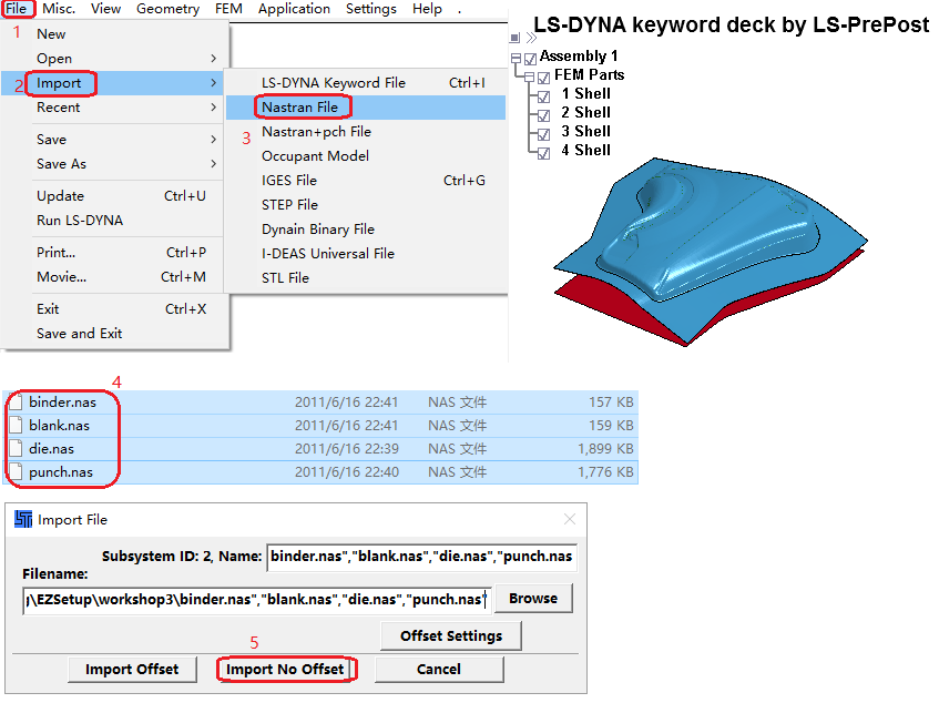
Open the menu.
Open the > menu.
Choose > > .
Select the binder.nas, blank.nas, die.nas, and punch.nas Nastran files.
Click .
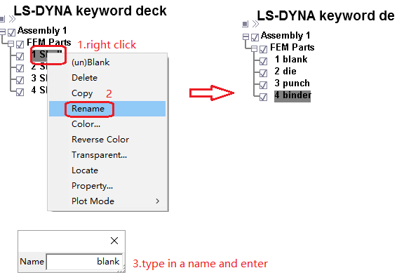
Right-click part 1, named Shell, in the parts tree to open the context menu.
Choose from the context menu.
Enter the name
blankand press Enter.Rename the other parts of the assembly
2 =
die.3 =
punch.4 =
binder.
.
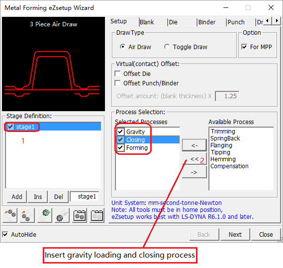
Choose > > from the menus.
In the Stage Definition section, click stage1.
In the Process Selection section, transfer the Gravity, Closing, and Loading processes from the Available list to the Selected list.
.
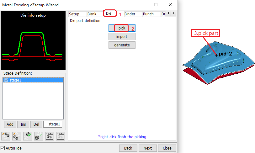
Continuing in the Metal Forming eZsetup Wizard:
Click the Die tab.
Click .
In the Graphics Window click the part (pid = 2) that is the die to pick it.
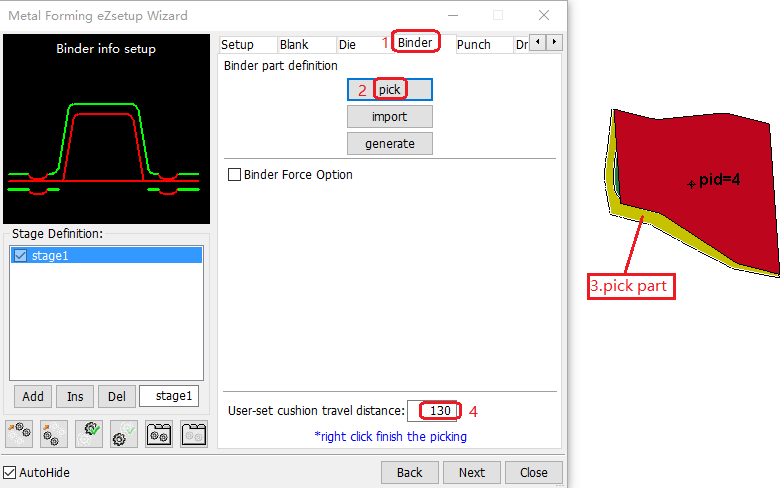
Continuing in the Metal Forming eZsetup Wizard:
Click the Binder tab.
Click .
In the Graphics Window click the part (pid = 4) that is the binder to pick it.
Set User-set cushion travel distance =
130.
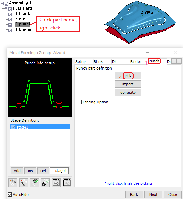
Continuing in the Metal Forming eZsetup Wizard:
Click the Punch tab.
Click .
In the parts list right-click the part name (3 punch) to pick it.
Continuing in the Metal Forming eZsetup Wizard:
Click the Blank tab.
Click .
In the Graphics Window click the part (pid = 1) that is the blank to pick it.
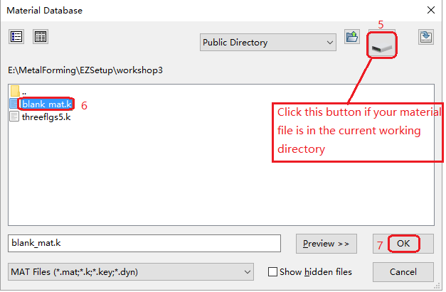
Click to open the Material Database window.
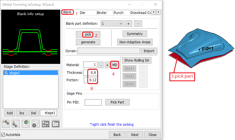
If the material file is in the current working directory, click the button.
Find the blank mat.k material file in the directory and select it.
Click .
Set Thickness =
0.9and Friction =0.12.
Choose > > from the menus, and import bead_lines.igs.
Then, in the Metal Forming eZsetup Wizard:
Click the Drawbead tab.
Click .
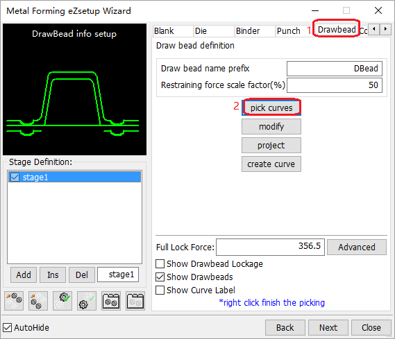
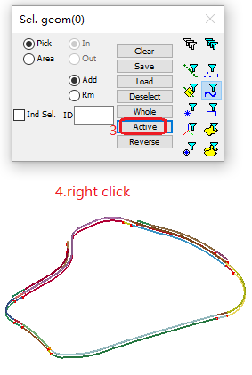
In the Sel. geom window click .
In the Graphics Window, right-click the imported bead lines to pick them.
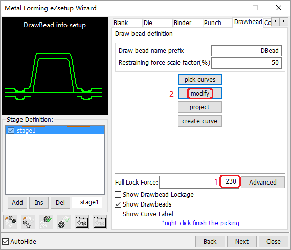
Continuing in the Metal Forming eZsetup Wizard's Drawbead tab:
Set Full Lock Force =
230.Click modify.
Click DBEAD6 in the DrawBead List.
Set the Force Scale Factor =
40.Click .
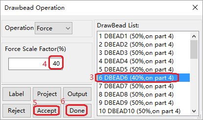
Repeat these steps for other Drawbeads until the factors are all set to the values shown in this table:
Drawbead Name Force Percentage (%) 1 DBead1 50 2 DBead2 50 3 DBead3 50 4 DBead4 50 5 DBead5 50 6 DBead6 40 7 DBead7 20 8 DBead8 10 9 DBead9 10 10 DBead10 10 11 DBead11 20 12 DBead12 20 13 DBead13 20 14 DBead14 20 15 DBead15 30 16 DBead16 30 17 DBead17 30 18 DBead18 30 Click .
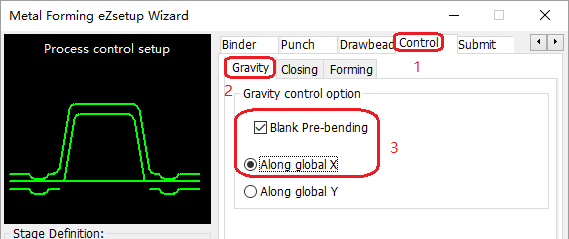
Continuing in the Metal Forming eZsetup Wizard:
Click the Control tab.
Click the Gravity sub-tab.
Activate Blank Pre-bending, and select Along global X.
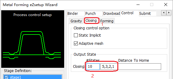
Continuing in the Metal Forming eZsetup Wizard's Control tab:
Click the Closing sub-tab.
Set #States=
10, and set Distance To Home=5,3,2,1.
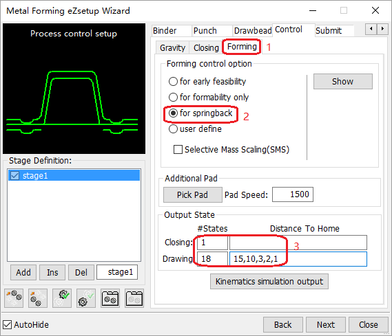
Continuing in the Metal Forming eZsetup Wizard's Control tab:
Click the Forming sub-tab.
Select .
Set Closing, #States=
1, set Drawing, #States=18, and set Drawing, Distance To Home=15,10,3,2,1.
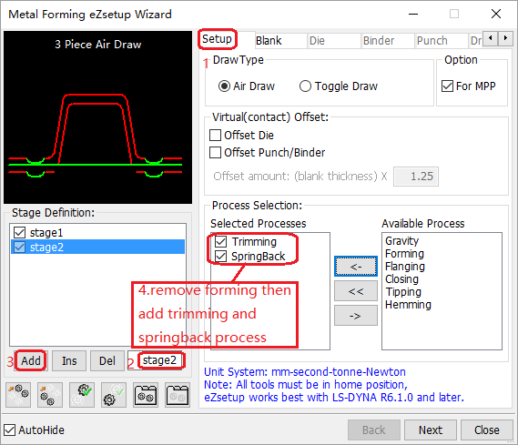
Continuing in the Metal Forming eZsetup Wizard:
Click the Setup tab.
Select .
Click .
Remove Forming from Selected Processes, then add Trimming and Springback.
Continuing in the Metal Forming eZsetup Wizard:
Click the Control tab.
Click the Trimming sub-tab.
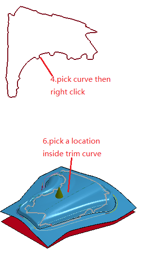
Click .
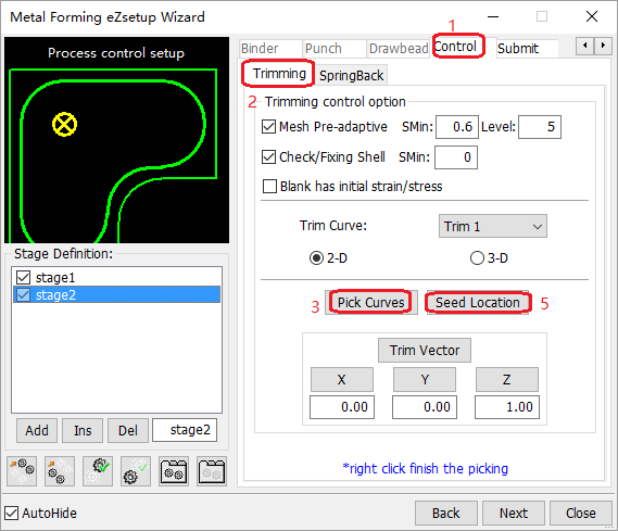
In the graphics window, pick the trim curve and then right-click it.
Click .
Pick a location inside the trim curve.
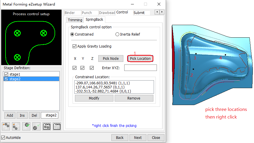
Continuing in the Metal Forming eZsetup Wizard's Control tab and Springback sub-tab:
Click .
Pick a location inside the trim curve.
Pick another location inside the trim curve.
Pick a final location inside the trim curve, then right-click.
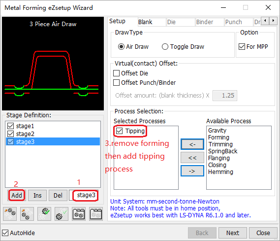
Continuing in the Metal Forming eZsetup Wizard's Setup tab:
Select .
Click .
Remove Forming from Selected Processes, then add Tipping.
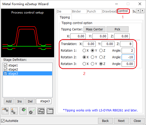
Continuing in the Metal Forming eZsetup Wizard:
Click the Control tab.
Enter the Translation, Rotation, and Angle values shown in the figure.
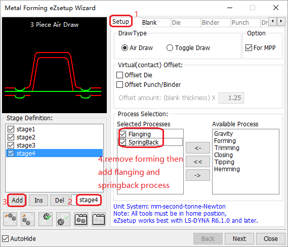
Continuing in the Metal Forming eZsetup Wizard:
Click the Setup tab.
Select .
Click .
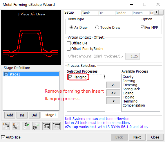
Remove Forming from Selected Processes, then add Flanging and Springback.
Import flanging tools:
Choose > > from the menus.
Select threeflgs5.k.
Click Import Offset.
Import flanging direction line:
Choose > > from the menus, and import flangingdir.iges.
Import pre-adaptive curve:
Choose > > from the menus, and import lineadp.iges.
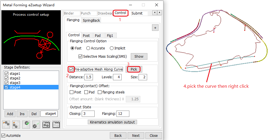
Continuing in the Metal Forming eZsetup Wizard:
Click the Control tab.
Activate Pre-adaptive Mesh Along Curve.
Click .
In the graphics window, pick the curve and then right-click it.
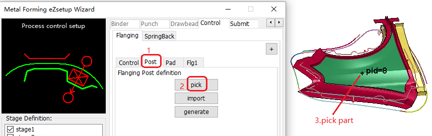
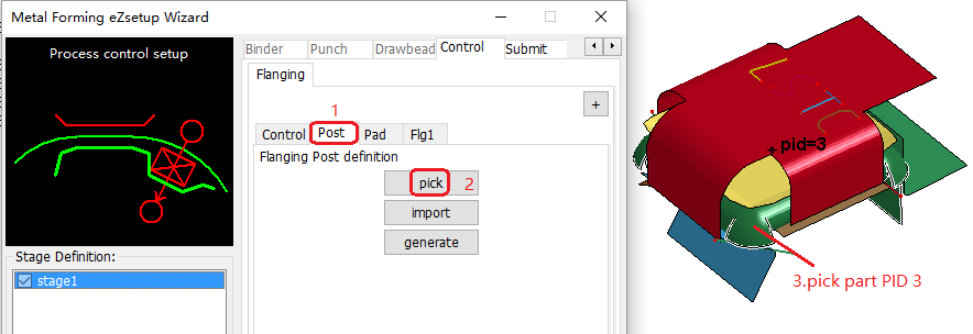
Continuing in the Metal Forming eZsetup Wizard's Control/Flanging tab:
Click the Post sub-tab.
Click .
In the graphics window, pick the part (pid=8).
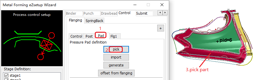
Continuing in the Metal Forming eZsetup Wizard's Control/Flanging tab:
Click the Pad sub-tab.
Click .
In the graphics window, pick the part (pid=6).
Continuing in the Metal Forming eZsetup Wizard's Control/Flanging tab:
Click the Flg1 sub-tab.
Click .
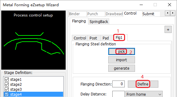
In the graphics window, pick the part (pid=9).
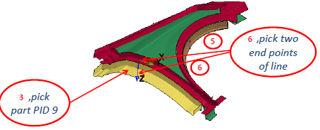
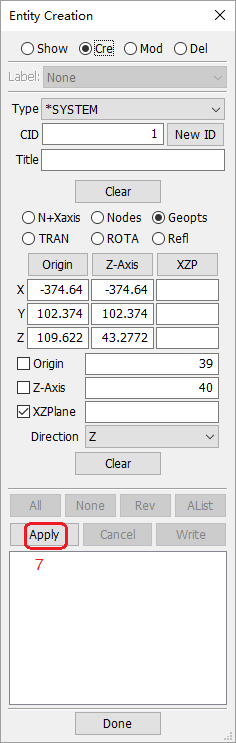
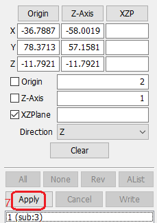
Click .
Pick one endpoint of the line.
Pick the other endpoint of the line.
In the Entity Creation window, click .
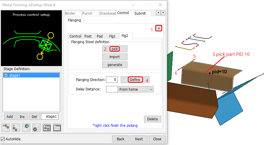
Continuing in the Metal Forming eZsetup Wizard's Control/Flanging/Flg2 tab:
Click +.
Click .
In the graphics window, pick the part (pid=10).
Click .
Repeat .
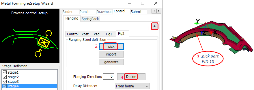
Repeat the steps in
to define one more flanging steel and their direction.
Continuing in the Metal Forming eZsetup Wizard's Control tab:
Click the SpringBack sub-tab.
Select the springback control option.
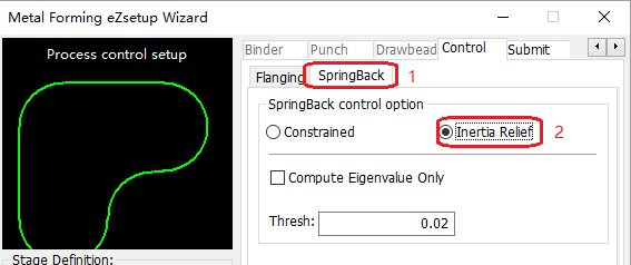
.
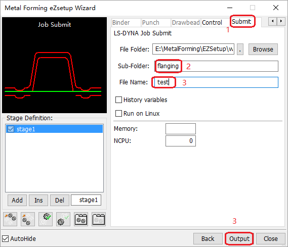
Continuing in the Metal Forming eZsetup Wizard:
Click the Submit tab.
Set Sub-Folder=
demo.Set File Name=
test.Click .
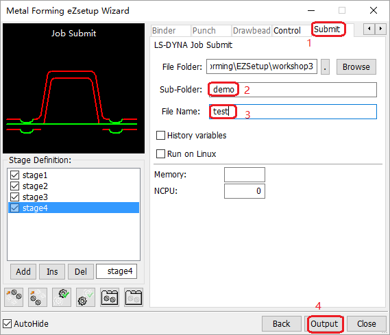
Submit test.bat to execute the LS-DYNA solver run.
Notes:
Simulations involving gravity, springback, and static implicit must use the double precision (DP) solver.
All other dynamic explicit simulation (for example, draw, or flanging) uses the SP solver.
The DP solver is slower than the SP solver.
Files required:
5_4_4_App_MF.zip: Download
Unit System:
mm-second-tonne-Newton
Import the blank and tools:
Choose > > from the menus.
Select blank.k and tools.k.
Click Import NoOffset.
Choose > > from the menus, and import FlangingVectors1_higherposition.iges.
Choose > > from the menus.
Remove Forming from Selected Processes, then add Flanging.
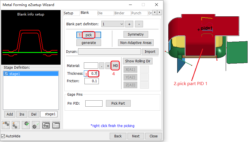
Continuing in the Metal Forming eZsetup Wizard's Blank tab:
Click .
In the graphics window, pick the part (pid=1).
Set Thickness=
0.7.Click .
In the Material Database window, open the Steel folder.
Open the BH180 folder.
Find and select the material file M37_Curve_BH180_NUMI2005Decklid.k.
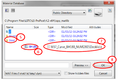
Click .
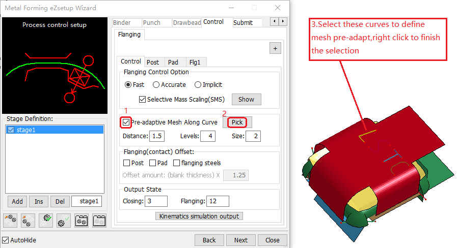
Continuing in the Metal Forming eZsetup Wizard's Control/Flanging/Control tab:
Activate Pre-adaptive Mesh Along Curve.
Click .
In the graphics window, select the curves indicated in the figure to define the mesh, then right-click to complete the selection.
Continuing in the Metal Forming eZsetup Wizard's Control/Flanging tab:
Click the Post sub-tab.
Click .
In the graphics window, pick the part (pid=3).
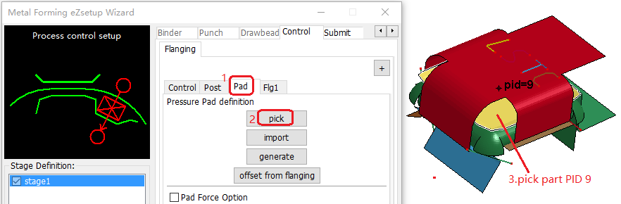
Continuing in the Metal Forming eZsetup Wizard's Control/Flanging tab:
Click the Pad sub-tab.
Click .
In the graphics window, pick the part (pid=9).
Continuing in the Metal Forming eZsetup Wizard's Contro/Flanging/Flg1 tab:
Click .
In the graphics window, pick the part (pid=8).
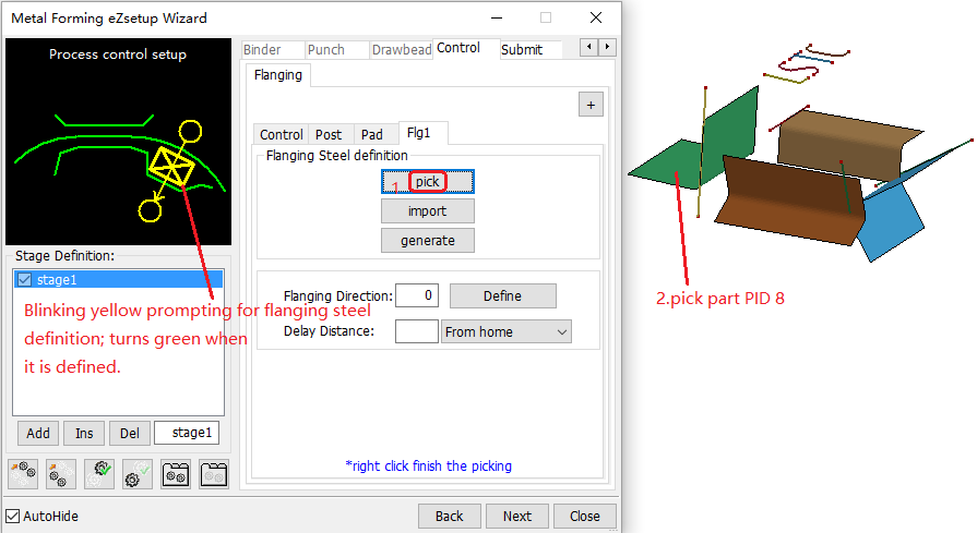
In the wizard, the flanging steel will blink yellow until it is defined, then it will be green.
Click .
Continuing in the Metal Forming eZsetup Wizard's Contro/Flanging/Flg2 tab:
Click .
Click .
In the graphics window, pick the part (pid=10).
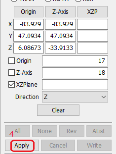
Click .
Pick one endpoint of the line.
Pick the other endpoint of the line.
Click .
Repeat these steps to define Flg3 and Flg4.
Continuing in the Metal Forming eZsetup Wizard:
Click the Submit tab.
Set SubFolder=
flanging.Set File Name=
testand then click .
Choose > > from the menus.
Set the Project name to
demo.Click .
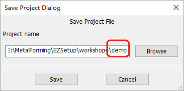
Note: The project file is an important database file, containing the complete model and EZSetup information. It can be reloaded back into LS-PrePost for changes in process or models.
Submit test.bat to execute the LS-DYNA solver run.
Note:
Simulations involving gravity, springback, or static implicit must use the double precision (DP) solver.
All other dynamic explicit simulations (for example,draw or flanging) use the SP solver.
The DP solver is slower than the SP solver.
Files required:
5_4_5_App_MF.zip: Download
Choose > from the menus.
Set File name=movie_000.
Click .
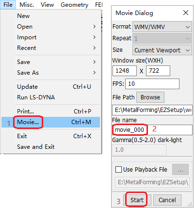
Note: Use MediaPlayer to open and play the movie file.
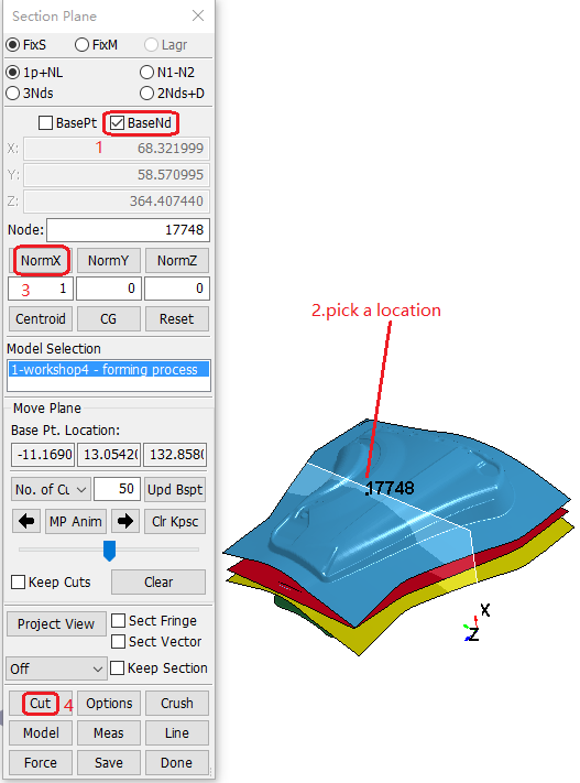
Choose > from the menus.
Activate BaseNd.
In the graphics window, pick a location.
Click .
Click .
.
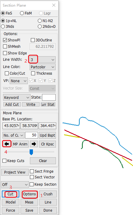
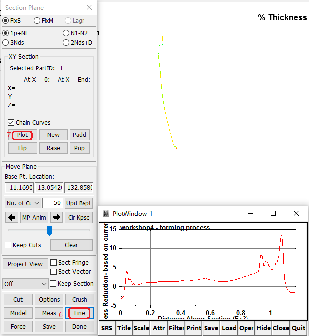
Continuing in the Section Plane panel:
Click .
Choose a Line Width of from the drop-down menu.
Click .
Click the left arrow next to .
.
Continuing in the Section Plane panel:
Activate Keep Cuts.
Click the left arrow next to .
Click .
Click .
Click .
.
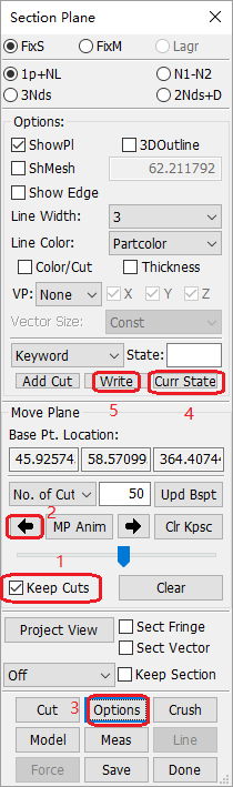
Note: Read in the saved cut sections into a fresh LS-PrePost session as keyword file, and check for the saved cuts. This is useful in springback measurement comparisons.
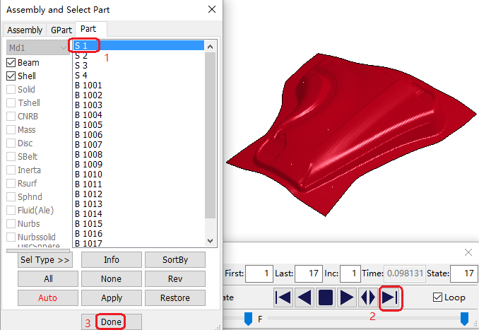
In the right tool bar, click , and then .
Select S 1.
Click the button.
Click .
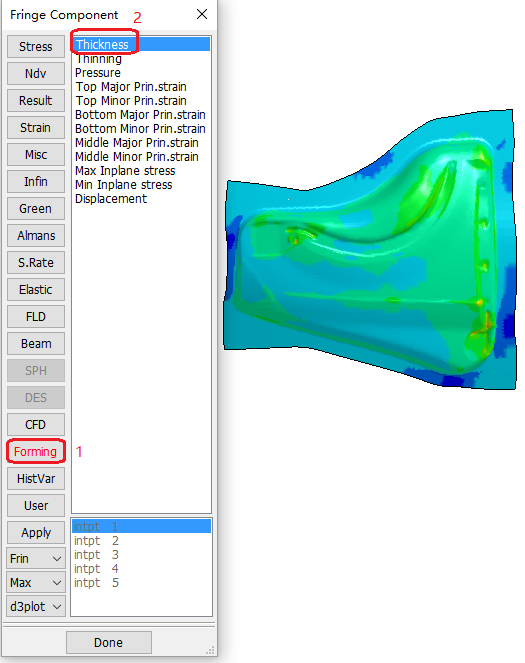
In the right tool bar, click , and then .
In the Fringe Component panel, click .
Select Thickness.
Click .
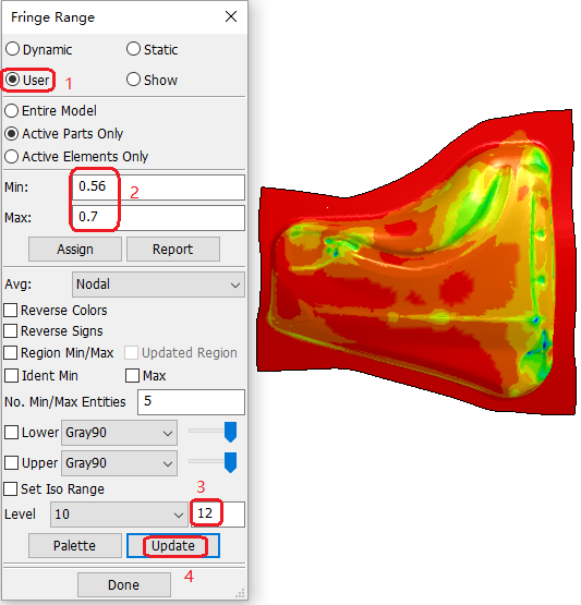
In the right tool bar, click , and then .
In the Fringe Range panel, select .
Set Min=
0.56and Max=0.7.Set Level=
12.Click .
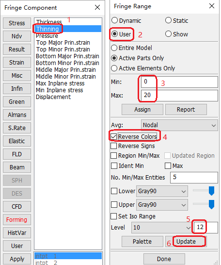
In the right tool bar, click , then , and select Thinning.
In the right tool bar, click , then , and select .
Set Min=
0and Max=20.Activate Reverse Colors.
Set Level=
12.Click .
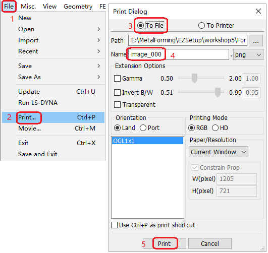
Open the menu.
Choose .
Select To File.
Set Name=
image_000.Click .
In the right toolbar click , then .
Select .
De-activate BaseND.
In the graphics window, pick a location close to the indicated node.
Click .
Click .
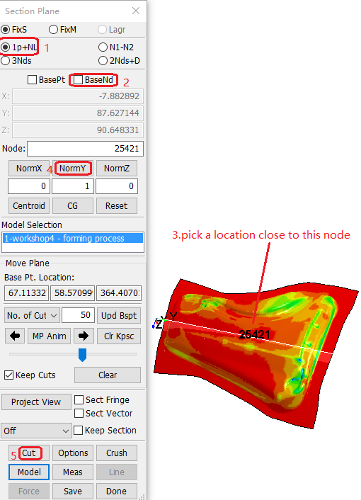
Click .
Click .
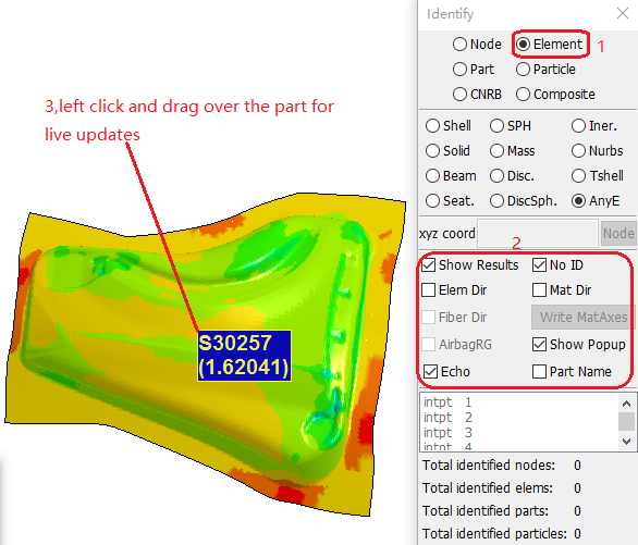
Open the Identify panel.
Select .
Activate and De-activate the additional options as shown in the figure.
In the graphics window, click the part to view values at that point.
Click-and-drag the pointer over the part to view constantly updated values.
In the right toolbar click , then .
Set t=
0.7.Set n=
0.21.Select .
Pick any location on the part (pid=1).
Choose from the Position drop-down menu.
Choose from the drop-down menu.
Click .
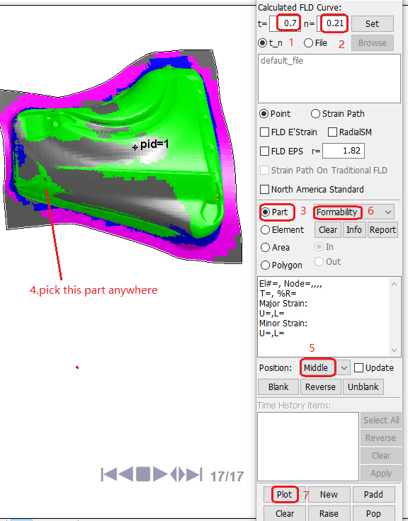
In the Formability Diagram dialog, set R-value=
1.82and press Enter.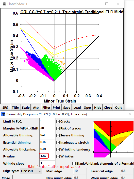
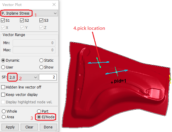
In the Vector Plot panel:
Choose from the drop-down menu.
Choose from the SF drop-down menu.
Select El/Node.
Pick a location on the part to display the strain vectors at that location.
.
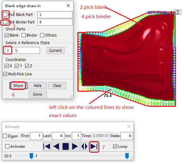
In the feature tree, deactivate parts until only the blank (1 S) and binder (4 S) are visible.
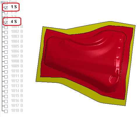
In the right toolbar, click then . In the Blank edge draw-in panel:
Activate Pick Blank Part.
In the graphics window, click the blank to pick it.
Activate Pick Binder Part.
In the graphics window, click the binder to pick it.
Set Select A Reference State=
1.Click .
In the Animate panel, click to display the final state of the formed part.
.
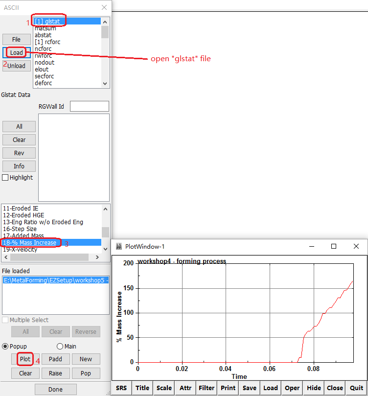
In the right toolbar, click then . In the ASCII panel:
Select rcforc.
Click to open the rcforc file.
Select Ma-1: die.
Select 3-Z-force.
Click .
.
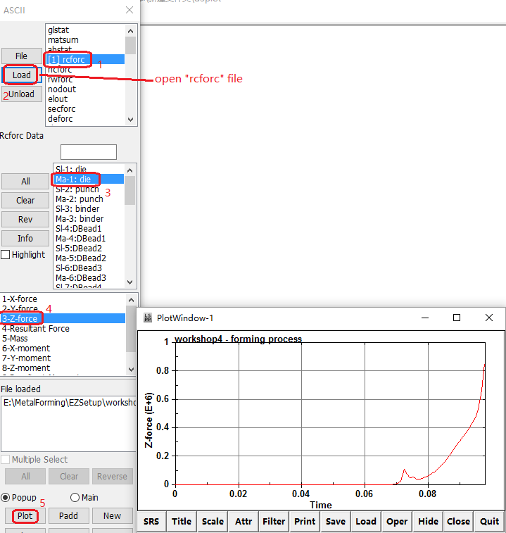
Note: 1 English ton = 8900 Newton.