The default bunching law. The two initial heights and ratios define parabolas in a coordinate system where the number of node points is the X-axis and the cumulative distance along the edge is the Y-axis. The parabolas are truncated where their tangent lines are identical; the spacing is linear between these points. If there are not enough nodal points to form this linear segment, a hyperbolic law is used and the ratios are ignored.

The Spacing1 and Ratio1 parameters define the distribution from the beginning of the edge to the midpoint of the edge using an Exponential law. Spacing2 and Ratio2 are similarly used to define the distribution from the terminating end of the edge to the midpoint of the edge.

The node spacing is described by the following equation:  

The parameters are computed according to the vertex constraints. If a ratio equals 0 at a vertex, the spacing constraint at this vertex only is taken into account and the ratio constraint with the neighbor spacing is left free by decreasing the polynomial order in the mathematical function.

The spacing of the node intervals is calculated according to the curvature of the function defining the distribution.

The spacing of the i'th interval from the beginning of the edge is defined using an exponential function of the Spacing1 and Ratio1 parameters.

The Exponential1 bunching law equation is as follows:  

where S_i is the distance from the starting end to node i, Sp1 is Spacing1, and R is the ratio given by 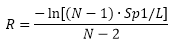 , where N is the total number of nodes and L is the total edge length.

Similar to Exponential1, except that Spacing2 and Ratio2 parameters are used and the distribution starting point is the terminating end of the edge.

Opens the Relative Point Density vs Edge Distance DEZ where you can graphically create a bunching law and immediately see it effects.

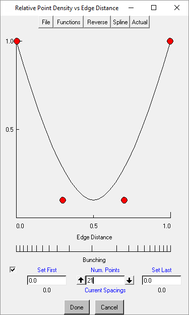
The top of the DEZ has a set of global menus.

The graphical display is a visual representation of the node density vs. edge distance. A higher y-coordinate will result in a higher node density. Control points may be moved (click and drag), added (click) or removed (double-click).

The Edge Distance display shows how the nodes will be distributed along the edge.

You may increase or decrease the number of nodes using the up or down arrows, or by manually entering an new value.

Enable the check box to manually set the location of the first and last nodes, if desired.

Use this law to seed the bunching using edge splits. For example, you can use Split Edge to split an edge arbitrarily. Then, if you apply this FromEdgeSplits bunching law to the split edge, you can interactively adjust the node distribution by editing the edge split locations (Edit Edge, Move Vertex, or similar).

The spacing of node intervals is calculated using the cosine function. The ends of the edge have the same constraint values for spacing and ratio.

The normalized distance from the starting node, t_i, is given by ,

where φ is found by a linear distribution of n-3 nodes over the range of to .

Spacing1 is used to set the first distance from the starting end of the edge, then the remaining nodes are spaced with a constant growth ratio. Only Spacing1 is specified.

The Geometric bunching laws are described by the following equation:  ,

where S_i is the distance from the starting end to node i, R is the ratio, and N is the total number of nodes. The ratio R is limited by 0.25 < R < 4.0.

Similar to Geometric1, except that Spacing2 is used to define the distribution starting from the terminating end of the edge.

The spacing pattern follows a half cycle of a Cosine function. Distribution begins from the starting point of the edge, and the parameters for spacing and ratio differ on either end.

The normalized distance from the starting node, t_i is given by ,

where φ is found by a linear distribution of n-3 nodes over the range of to .

Similar to HalfCosinus1 in that the parameters for spacing and ratio follow a half cycle of a Cosine function, but a sin function is used to perform the calculation to make the distribution appear to start at the terminating end.

The spacing parameters for each end are used to define a hyperbolic distribution of the nodes along the edge. You can set Spacing1 and Spacing2, and the growth ratios are determined internally.

The following equations are the basis for the Hyperbolic Tangential bunching law. After an initial distribution is calculated, iterative adjustments are applied for smoothing and tolerance checking.

The parameter limitations are:

The spacing of the node intervals is calculated using a linear function.

Use this option to manually adjust node placement by dragging along the selected edge.

The spacing of the node intervals is calculated according to a Poisson distribution. Requested values of Spacing1 and Spacing2 are used. Requested values of Ratio1 and Ratio2 are not used directly, but are used to determine if the requested spacing is appropriate. If not, the spacing will be adjusted automatically.

The mapping function is obtained by solving the following differential equation:

 ,

with the following boundary conditions:

 ,

where Sp1 = Spacing1 and Sp2 = Spacing2.

The function P is required to satisfy the Neumann boundary condition. It is computed by an iterative optimization process loop. Some parameter limitations are:

0.0 < Sp2 < 1.0

0.0 < Sp1 < 1.0 - Sp2

500 < Number of iterations < 9999

The node spacing is derived from an existing mesh edge distribution. This may be useful to seed an unstructured or swept face to obtain a better quality mesh, or to set up node for node contact with a preexisting unstructured mesh.

To use this option, an unstructured mesh must be loaded and the mesh edge must match the blocking edge, including associations to surrounding curves. Nodes Locked is enabled when this law is applied.

If the node distribution is changed on the reference edge (for example by splitting), then the PreMesh will go out of date and will have to be recomputed.

The spacing of the node intervals is calculated by an mspline function.

The nodes along the edge are uniformly distributed.