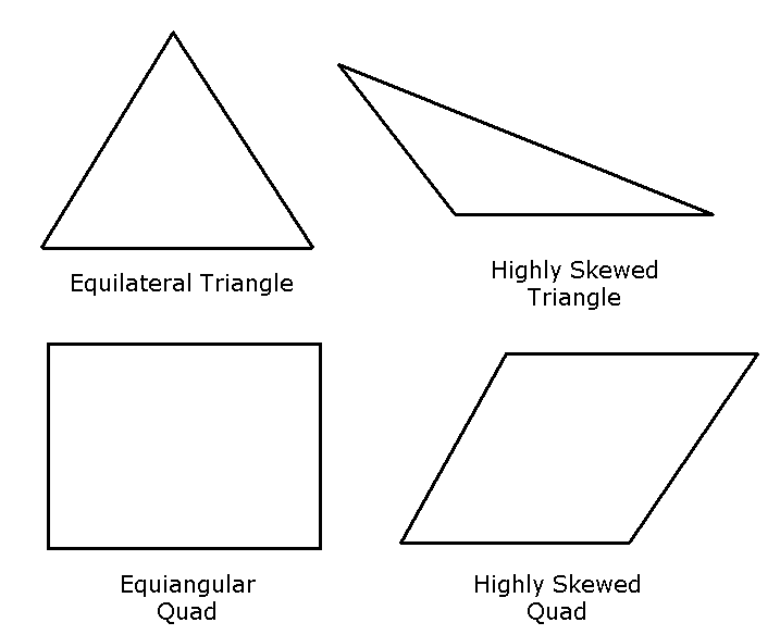
Skewness is one of the primary quality measures for a mesh. Skewness determines how close to ideal (that is, equilateral or equiangular) a face or cell is (see Figure 35.33: Ideal and Skewed Triangles and Quadrilaterals).
Note: Table 35.1: Skewness Ranges and Cell Quality lists the range of skewness values and the corresponding cell quality.
Table 35.1: Skewness Ranges and Cell Quality
| Value of Skewness | Cell Quality |
|---|---|
| 0 | degenerate |
| < 0.02 | bad (sliver) |
| 0.25 - 0.02 | poor |
| 0.5 - 0.25 | fair |
| 0.75 - 0.5 | good |
| 0.75 - 1 | excellent |
| 1 | equilateral |
According to the definition of skewness, a value of 1 indicates an equilateral cell (best) and a value of 0 indicates a completely degenerate cell (worst). Degenerate cells (slivers) are characterized by nodes that are nearly coplanar (collinear in 2D).
Highly skewed faces and cells are unacceptable because the equations being solved assume that the cells are relatively equilateral/equiangular.
Two methods for measuring skewness are:
Based on the equilateral volume (applies only to triangles).
Based on the deviation from a normalized equilateral angle. This method applies to all cell and face shapes, for example, pyramids and prisms.
The skewness method is equiangular for every element type.
Equilateral-Volume-Based Skewness
In the equilateral volume deviation method, skewness is defined as
 | (35–3) |
where, the optimal cell size is the size of an equilateral cell with the same circumradius.
Table 35.1: Skewness Ranges and Cell Quality provides a general guide to the relationship between cell skewness and quality.
The presence of cells that are fair or worse indicates poor boundary node placement. You should try to improve your boundary mesh as much as possible, because the quality of the overall mesh can be no better than that of the boundary mesh.
In 3D, most cells should be good or better, but a small percentage will generally be in the fair range and there are usually even a few poor cells.
Skewness-Normalized Equiangular
In the normalized angle deviation method, skewness is defined (in general) as
 | (35–4) |
where
Θmax = largest angle in the face or cell
Θmin = smallest angle in the face or cell
Θe = angle for an equiangular face/cell (for example, 60 for a triangle, 90 for a square)
For a pyramid, the cell skewness will be the maximum skewness computed for any face. An ideal pyramid (skewness = 1) is one in which the 4 triangular faces are equilateral (and equiangular) and the quadrilateral base face is a square. The guidelines in Table 35.1: Skewness Ranges and Cell Quality apply to the normalized equiangular skewness as well.
The procedure for checking the skewness is as follows:
Open the Mesh control panel by selecting Generate mesh in the Model menu, or by clicking the
 button in the Model and solve toolbar.
 Model
 Generate mesh
 Click on the Quality tab to show the mesh diagnostic tools.
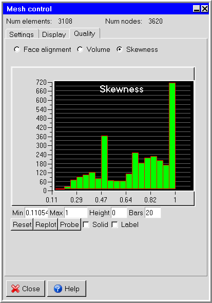
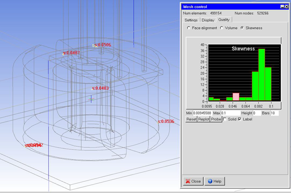
Select the Skewness option. Ansys Icepak will show a histogram of the skewness, as shown in Figure 35.34: The Skewness Histogram in the Mesh control Panel.
If you want to modify the range of skewness viewed, enter a new value in the Min or Max field and then press the Enter key on your keyboard or click Replot to update the histogram. To modify the maximum height of the bars or the number of bars in the histogram, enter a new value in the Height and/or Bars fields and click Replot. (Note that a Height of
0instructs Ansys Icepak to display the bars of the histogram at their full height.) To return to the default ranges, click the Reset button.To view the elements of the mesh within a particular range of skewness, click on a bar in the histogram, Ansys Icepak will display the elements in the selected range in the graphics window. Select the Solid option if you want to view these elements with solid shading. Select the Label option to show the corresponding skewness values.
If you want to find out which object the element belongs to, click on Probe. Use the left-mouse button to select any element in the graphics window. The corresponding object name will be shown in the graphics window momentarily as well as printed to the text window. To exit the probe mode, click middle or right mouse button.