The following sections of this chapter are:
This tutorial is divided into the following sections:
The current section describes how to setup and run a sequence of airflow mesh adaptation cycles within Fluent Icing. For this purpose, the ONERA M6 wing under transonic fully turbulent condition (M = 0.84 and Re = 11.8 million) is used. Despite the simple geometry, a lambda-shock develops over the suction side of the wing. The computational domain of the ONERA M6 wing is made of 1,533,678 nodes and 4,266,117 cells. The wing surface is discretized by approximately 99,000 triangles and the height of the first layer of cells guarantee a Y+ that is below 1 under this condition.
A mesh, such as this one, is considered relatively coarse to capture shocks. Therefore, this tutorial will demonstrate how a sequence of airflow mesh adaptation cycles improves the level of precision of CFD results by capturing not only the lambda shock, but also the wake and wing tip vortex produced by the ONERA M6.
This tutorial is divided into two sections:
Initial Fluent Airflow Simulation: This section shows how to setup a clean transonic airflow simulation using Fluent Icing and its corresponding Fluent Solution session that is suitable for mesh adaptation.
Mesh Adaptation Cycles: This section demonstrates how to configure Fluent Icing to perform 2 airflow mesh adaptation cycles. Each cycle is composed of an airflow (Fluent) and mesh adaptation (OptiGrid) solver. For more information regarding OptiGrid, see OptiGrid - Mesh Adaptation within the FENSAP-ICE User Manual.
Download the fluent_adaptation.zip file
here .
Unzip fluent_adaptation.zip, preferably inside your working directory.
In this section, you will learn how to set-up a clean transonic airflow simulation within Fluent Icing and its corresponding Fluent Solution session. The latter will allow you to access Fluent settings that are not exposed inside Fluent Icing and that enhance the quality and accuracy of your airflow and adapted mesh results.
The table below shows the transonic conditions of this tutorial. These conditions yield a Mach number of ~0.84 and a Reynolds number of ~11.8 million.
Table 38.1: Transonic Condition
| Characteristic Length (MAC) | 0.65 m |
| Speed | 269 m/s |
| Angle of Attack (α) | 3.06 ˚ |
| Pressure | 80,600 Pa |
| Temperature | 255 K |
Launch Fluent 2024 R2 on your computer.
Use the Fluent Launcher to start Ansys Fluent.
In the Fluent Launcher, set the Capability Level to Enterprise, then select Icing.
Set Solver Processes between
8and12.Click Start.
Alternatively, Fluent Icing can be opened using the icing (on Linux) or icing.bat (on Windows) file inside the fluent/bin/ folder.
Once Fluent Icing opens, the Project tab will be displayed. In the Project’s top ribbon panel, select Project → and enter
OneraM6_Adaptationto create a new Project folder.Note: A Fluent project allows you to save and manage multiple simulations and runs in a single project folder.
From the top ribbon panel, go to File and select . In the Preferences window, select Icing.
Click and to display the Fluent Solution session user interface, including its Graphics window, that is connected to Fluent Icing.
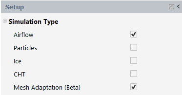
Enable . Mesh adaptation is a hidden feature that only appears in the graphical user interface of Fluent Icing when are active.
Click to access extra smoothing parameters that will be used during mesh adaptation.
Press .
Go to
 Project
→ Simulation → Import
Case and browse to
fluent_adaptation/workshop_input_files/Input_Grid
and select the oneram6.cas.h5 file from the
extracted fluent_adaptation.zip archive.
Project
→ Simulation → Import
Case and browse to
fluent_adaptation/workshop_input_files/Input_Grid
and select the oneram6.cas.h5 file from the
extracted fluent_adaptation.zip archive.A New Simulation window will appear. Enter the Name of the new simulation as
oneram6_adaptation, and check to enable this option. Press .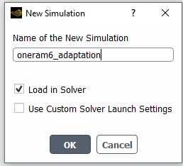
A new Fluent Solution window will appear. This window is connected to your Fluent Icing window. Minimize this window to proceed.
Within Fluent Icing, a new simulation folder will be created within the Project View, and the oneram6.cas.h5 file will be imported. You should now see the oneram6_adaptation (loaded) tree under the Outline View.
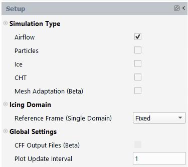
Select the Setup tree menu under oneram6_adaptation (loaded) and in the Setup panel, check . Disable all other simulation types.
Continue further down and right-click the Airflow tree menu located under Setup and select to make sure the previously Fluent simulation settings are properly transferred to Fluent Icing.
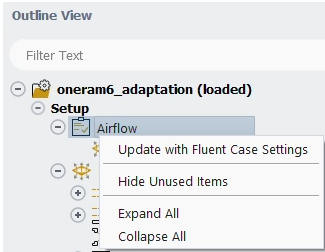
Click Setup → Airflow to display the Airflow panel.
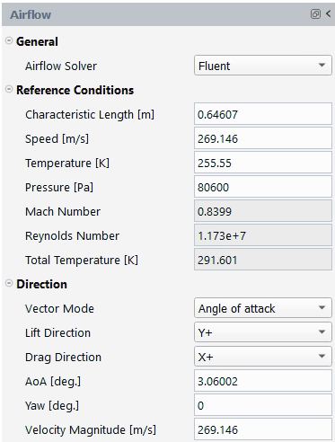
Under General, select as the Airflow solver.
Under Reference Conditions, ensure the airflow conditions correspond to the transonic conditions mentioned in Table 38.1: Transonic Condition. To work in absolute pressure, set Pressure [Pa] to
0. Verify that these conditions satisfy the Mach Number of ~0.84 and Reynolds Number of ~1.18 million at the bottom of this panel.Under Direction, go to Vector Mode and select to specify the orientation of the reference airflow. Set the Lift Direction and Drag Direction to and respectively. Set the AoA [deg.] to
3.06and the Velocity Magnitude [m/s] to269(Table 38.1: Transonic Condition).
Click Setup → Airflow → Fluent to display the Fluent panel.
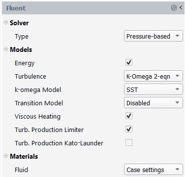
Under Solver, set Type to .
Under Models, ensure that , and are enabled, that Turbulence is set to and k-omega Model to .
Under Materials, select next to Fluid. This will use the fluid properties of your case file. By default, Fluent Icing only uses constant air properties. In transonic regimes, these properties are not constant. Therefore, to improve accuracy, you will later select temperature dependent air properties inside the Fluent Solution window that is connected to Fluent Icing.
Go to Setup → Boundary Conditions,
Inside Inlets, click pressure-far-field-4 to display its properties panel.
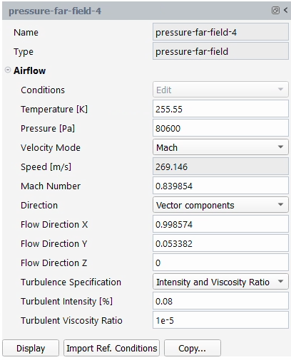
Under Airflow, select next to Conditions.
Go to the bottom of this panel and click . This will copy the Reference Conditions set inside the Airflow panel as boundary conditions.
Inside Walls, select wall-5 boundary,
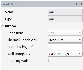
Under Airflow,
Set Thermal Conditions to and impose a Heat Flux [W/m2] of
0.Set the Wall Roughness to ; all the walls inside the case file were set to
0Roughness Height [m].
Repeat the process described above for wall boundaries wall-6 and wall-7. All wall surfaces of the ONERA M6 are adiabatic and smooth.
Go to the Fluent Solution window that is connected to Fluent Icing and, inside its Outline View,
Double-click Setup → Materials → Fluid → to display the material properties of air.
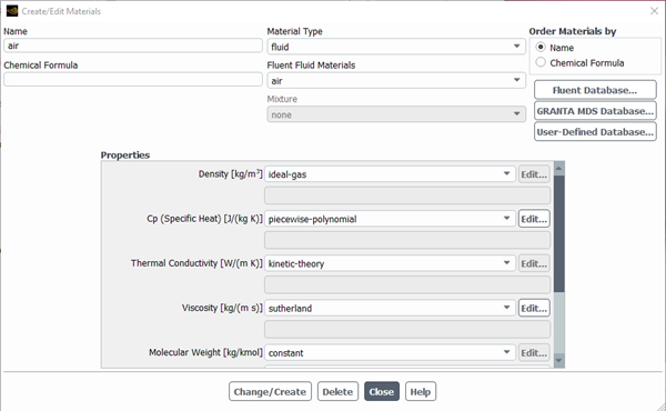
Under Properties,
Set Density [kg/m3] to .
Set Cp (Specific Heat) [J/kg K)] to .
A Piecewise-Polynomial Profile dialog will open. Press to accept all default settings.
Set Thermal Conductivity [W/(m K)] to .
Set Viscosity [kg/(m s)] to .
A Sutherland Law dialog will open. Press to accept all default settings.
Leave the other properties as they are. Click to save your changes. Click to proceed.
Note: These air properties are temperature dependent and have been used in a wide variety of validation cases.
Go to Setup → Boundary Conditions → Wall
Select wall-5 and wall-6 while pressing the Ctrl key. This automatically selects these two boundary surfaces.
Right-click wall-6, a submenu appears. Select to combine these 2 wall surfaces into one.
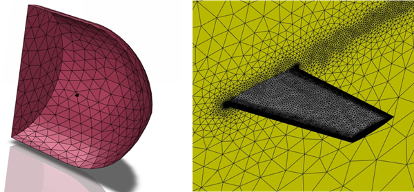
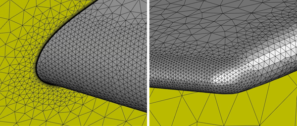
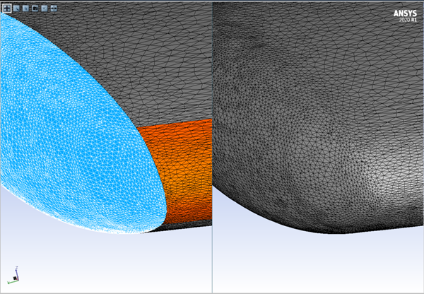
Note: wall-5 and wall-6 represent the upper and lower surfaces of the ONERA M6 wing. They meet at the leading edge of the wing where the curvature is expected to be continuous. CAD surfaces created internally by OptiGrid for node projection will have discontinuous curvature across this edge, which may produce a visible crease in the mesh after adaptation. To avoid this, such edges can be removed by combining their associated surfaces before mesh adaptation. See the figure below for an example of mesh adaptation with and without this merging step. Wall-7 should not be merged with the other walls as its surface represents a blunt trailing edge and the curvature between the wing and its trailing edge is discontinuous.
Double-click wall-7 and, inside its Wall panel, change its Zone Name to . Click to save your changes. Click to proceed.
Double-click wall-5 or wall-6 (automatically generated surface name given by Fluent after the merge) and, inside its Wall panel, change its Zone Name to wing. Click to save your changes. Click to proceed.
Figure 38.3: Surface Mesh at the Wing Tip After One Mesh Adaptation: Without (Left) And With (Right) Merging Wall Surfaces
Note: The imported case file has been set to obtain a robust Pressure-Based 2nd order airflow solution and to monitor convergence of lift and drag coefficients. In this manner,
Inside Setup → Reference Values, the Area [m2] is set to 0.7728935 in order to compute the aerodynamic coefficients.
Inside Solution → Methods, the Pressure-Velocity Coupling scheme is set to . In Spatial Discretization, the Gradient is set to and the remaining options to or . A Pseudo Time Method is selected, and the High Order Term Relaxation option is enabled to improve convergence.
Inside Solution → Controls, the explicit relaxation factors are set to 0.5 for all parameters except Density, which is set to 1.
Inside Solution → Initialization → , have been enabled in Initialization Options.
Inside Solution → Run Calculation, the Time Scale Factor of the Conservative Length Scale Method has been reduced to 0.05.
This setup is used as is by Fluent Icing.
Go back to the Fluent Icing window and right-click symmetry-8 under Setup → Boundary Conditions → Other. Select to sink the boundaries of Fluent Icing with those of Fluent Solution and to reflect the merge and the renaming of wall boundaries.
In the ribbon, go to and select to save your changes to the oneram6.cas.h5 file. This will save your mesh topology changes that will be later used by the mesh adaptation solver.
Inside the Outline View, select Airflow under Solution. Inside the Airflow panel, set Number of Iterations to
500and press .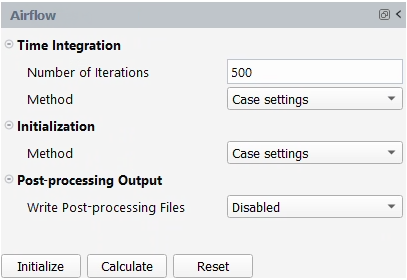
A New run window will appear. Set the Name of the new run to
flow_origand click . The calculations will start with hybrid initialization.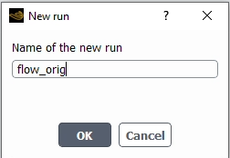
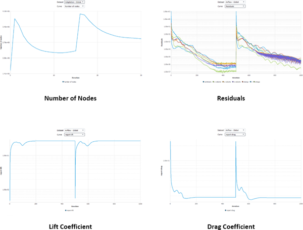
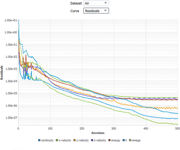
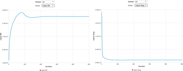
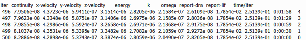
Monitor the convergence of this calculation inside Fluent Icing. Go to the window located at the right of your Fluent Icing window and look at the residuals and aerodynamic coefficient curves. The following three figures show the convergence of residuals and lift and drag coefficients as well as their values at the end of the simulation. After 500 iterations, lift and drag coefficients should have converged to the following values ~0.2514 and ~0.01785 respectively.
Once the computation is complete, an Airflow icon will appear under the flow_orig run folder in the Project View. This icon shows that a solution has been obtained and has been saved inside the run directory, flow_orig. The solution is oneram6.dat.h5.
Go to Project View and right-click the Airflow icon located inside the flow_orig run folder. Choose → . This will open the flow solution using Viewmerical.
In Viewmerical, follow these steps to output the pressure coefficient and mach number.
Pressure coefficient
To create contours along the surface of the wing and at the symmetry plane (Z = 0 m).
Inside the Objects panel, disable . Enable , and .
Inside the Data panel, set Data to and change the Color range to .
To create contours along the surface of the wing and at Z = 0.75 m.
Inside the Objects panel, disable and . Enable and . Go to the submenu, select and set Pos to
0.75.Inside the Data panel, set Data to and change the Color range to .
2D plots along the wing at Z = 0 m and Z = 0.75 m.
Inside the Query panel, set 2D Plot to .
Make sure that Target is set to and that Cutting plane is set to .
Select as the horizontal axis. To do so, set in the bottom left corner of your plot.
Set the text box to the right of Cutting plane to
0and0.75to see the pressure coefficient along the wing at Z = 0 m and Z = 0.75 m respectively.
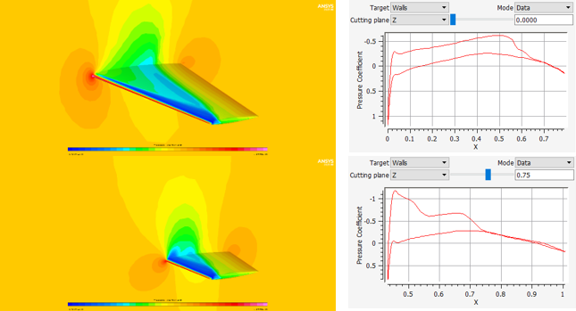
The image below shows the post-processed figures described in the previous steps.
Figure 38.7: Pressure Coefficient Contours and 2D Plots at Z = 0 m Plane (Top) and Z = 0.75 m Plane (Bottom)
Mach number
To create contours at the symmetry plane (Z = 0 m).
Inside the Objects panel, disable , and . Enable .
Inside the Data panel, set Data to and change the Color range to .
To create contours at Z = 0.75 m.
Inside the Objects panel, disable , , and . Go to Cutting Plane submenu, select and set Pos to
0.75.Inside the Data panel, set Data to and change the Color range to .
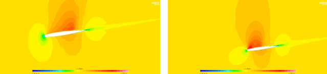
The image below shows the post-processed figures described in the previous steps.
As observed in the previous pressure coefficient and mach figures, the coarse mesh was able to roughly capture the lambda shock of the airflow. The sharp pressure drop across the shocks is not well represented nor is the airflow around the wing and at the wake. Also, mach number contours reveal too much numerical noise in the solution. In the next section, you will use mesh adaptation cycles to improve this solution.
Close Viewmerical without closing Fluent Icing.
In this section, you will learn how to set-up a sequence of mesh adaptation cycles from an existing airflow solution in order to improve its precision. In this case, two (2) cycles are sufficient to better capture the pressure drop across the lambda shock, the airflow acceleration along curved surfaces such as the leading edge and the wing tip, and the wake produced by the wing.
Note: Inside Fluent Icing, mesh adaptation is done using Ansys OptiGrid. The latter allows anisotropic mesh optimization by aligning and stretching cells and edges with flow features to minimize and homogenize the Hessian-based mesh error of selected solution fields. Only unstructured meshes (prisms and tetrahedrons) are supported. Several mesh operations are done to reduce this error: mesh coarsening, mesh refinement, edge swapping and node movement. The most relevant parameters of Ansys OptiGrid are exposed in Fluent Icing. For more information, see OptiGrid - Mesh Adaptation within the FENSAP-ICE User Manual.
After you obtain the airflow solution in Initial Fluent Airflow Simulation, in the Outline View of Fluent Icing, select Setup under oneram6_adaptation (loaded). In the Setup panel, enable and make sure that is also enabled. This will automatically create a Mesh Adaptation entry under Setup and Solution.
Go to Setup → Mesh Adaptation.
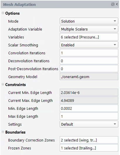
Click , located at the bottom of the panel, to create a CAD from the mesh of the oneram6.cas.h5 file. This CAD contains the surfaces that bound the computational domain and is used as the geometry to preserve in all mesh adaptation cycles.
Note: Since the CAD is reconstructed from the initial mesh, it is important that this mesh possesses a high surface mesh resolution on rounded surfaces. This will improve the accuracy of the generated CAD. In the current tutorial, this has not been done in order to reduce mesh size and therefore computational time and resources.
Under Options,
Set Mode to to conduct mesh adaptations using airflow solutions.
Set Adaptation Variable to .
In Variables, select , , , , , and . The first 6 fields represent the primitive variables of the airflow solver. The turbulent viscosity is a post-processed field predicted by the turbulence model. Press .
Set Scalar Smoothing to . This gives you access to parameters that remove numerical noise or enhance flow discontinuities.
Set Convolution Iterations to
1. Convolution is used to filter the solution and remove numerical noise. A value of one represents the number of time steps required to solve a Laplacian equation that smooths the solution fields. This is usually required when the original grid is coarse, which is the case in this tutorial.Keep Deconvolution Iterations and Post-Deconvolution Iterations to
0.
Under Constraints,
Take a moment to look at the Current Min. Edge Length and Current Max. Edge Length of the original ONERA M6 mesh. OptiGrid provides these lengths as guidelines to set the minimum and maximum edge length constraints to respect during mesh adaptation.
Set the Min. Edge Length of cells to
2e-4. This represents approximately a tenth of the thickness of the trailing edge at the wing tip. This is the smallest geometric dimension along the wing and should be enough to highlight the surface mesh refinement improvements made specially at the leading edge of the wing and along the shock.Set the Max. Edge Length of cells to
1. This represents approximately a fifth of the current maximum length that is located at farfield. Reducing the maximum length of cells at farfield will improve the transition in mesh refinement between the wing and the farfield as mesh adaptation cycles are executed.Keep Settings as .
Under Boundaries,
In Boundary Correction Zones, select trailing-edge and wing. This will preserve the prism layer height and growth ratio of the walls selected.
In Frozen Zones, select trailing-edge to prevent surface mesh adaptation on the trailing edge of the ONERA M6. This surface has been specified as a frozen zone to reduce the mesh size of adapted meshes and to show its functionality.
Go to Solution and under Mesh Adaptation (beta), set Number of Solver-Adaptation Loops to
2. This will allow you to conduct two adaptation cycles. Each cycle or loop is composed of an adapted mesh and its corresponding airflow solution.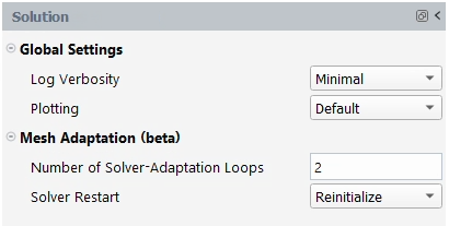
Go to Solution → Mesh Adaptation.
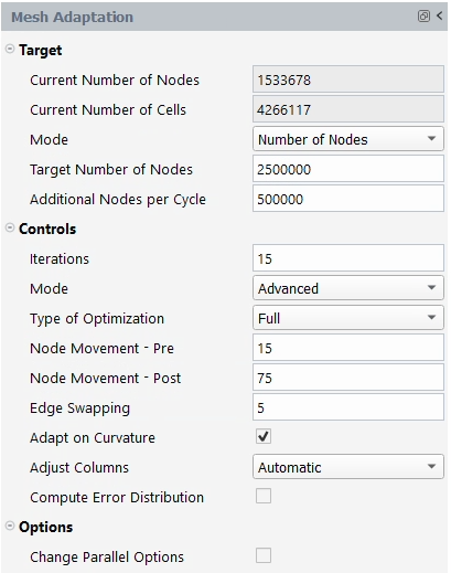
Under Target,
Take a moment to look at the Current Number of Nodes and Current Number of Cells of the ONERA M6 mesh. OptiGrid provides these numbers as guidelines to control the mesh size per mesh adaptation cycle.
Set Mode to to control the size of the adapted meshes.
Set Target Number Nodes to
2,500,000to set the target number of nodes of the first adapted mesh.Set Additional Nodes per Cycle to
500,000to set the number of nodes to add at each mesh adaptation cycle after the first adapted mesh.
Under Controls,
Set Iterations to
15. In this manner, fifteen mesh adaptation iterations will be carried out per mesh adaptation cycle.Set Mode to . New options appear that will allow you to control the type of mesh optimization and the number of mesh movement operations per iteration.
Set Type of Optimization to . In this mode, all supported mesh operations (add/remove nodes, edge swapping and node movement) can be performed.
Set Node Movement – Pre to
15. This sets the maximum number of node movement, edge refinement and swapping loops to smooth and optimize the mesh based on different constraints per iteration.Set Node Movement – Post to
75. This sets the maximum number of node movement loops to smooth the adapted mesh per iteration.Set Edge Swapping to
5.Enable and disable Compute Error Distribution.
Note: Compute Error Distribution is currently supported for single mesh adaptations.
In the Outline View, right-click Solution and select . A New run window will appear. Set the Name of the new run to
adapt_loop_oneram6. Press .
Monitor the convergence of this calculation inside Fluent Icing. Go to the Plots window located at the right of your Fluent Icing window and look at convergence plots of mesh adaptation and airflow by navigating through the Dataset list. and contain the convergence history of all adaptation cycles per solver. Inside this list, numbers displayed next to Adaptation or Airflow link an adaptation cycle to its corresponding convergence plot.
The following figures show the convergence of the number of nodes, residuals and lift coefficient during adaptation cycles.
As the mesh size increases and regions become finer with mesh adaptation, the initial convergence settings, in this case, the time scale factor and the relaxation parameters, should be adjusted and become more robust in order to guarantee good convergence of the airflow solver throughout the mesh adaptation cycles/loops. In this tutorial, a time scale factor of 0.05 guarantees a good convergence of the airflow within 500 iterations as residuals are below 1e-5 and lift and drag coefficients plateaued. The table below shows the lift and drag coefficients produced by the original mesh and each mesh adaptation cycle.
Table 38.2: Aerodynamic Coefficients during Mesh Adaptation Cycles
CL ΔCL CD ΔCD Original Mesh 0.251391
---
0.017854
---
1st Adapted Mesh 0.264926
5.38%
0.018516
3.71%
2nd Adapted Mesh 0.266362
0.54%
0.018207
1.67%
This table shows that differences in lift and drag coefficients between successive adapted meshes decay with mesh adaptation.
Note: If more adaptation cycles are sought, for instance to reduce the difference in drag coefficient below 1%, the time scale factor of the airflow solver should be further reduced and its number of iterations per cycle should increase consequently. Moreover, you should either increase the number of adaptation iterations per cycle and/or to increase the number of node movement pre- and post- iterations to guarantee a smooth mesh during adaptations.
If accurate mesh independent solutions are sought, enable surface mesh adaptation at the trailing edge. This will require a larger target number of nodes.
Once all simulations are completed, load the two adapted solutions and the original solution inside Viewmerical. To do this, go to Project View and,
Right-click the Airflow file located inside the flow_orig subfolder. Select → .
Right-click the Airflow file located inside the adapt_loop_oneram6/out_01 subfolder. Select → . A message asking if you would like to append this solution to Viewmerical will appear. Click to load this solution into the same Viewmerical window that contains the original solution.
Repeat the above step for the Airflow solution file located inside the adapt_loop_oneram6/out_02 subfolder.
Rename the first solution that was loaded to
orig, the second to1st_adaptand the third to2nd_adapt. Compare pressure coefficient contours over the wing, symmetry plane and the Z = 0.75m plane betweenorigand2nd_adaptsolutions. Enable and in Object to see the contours in standalone mode and contours with their respective surface mesh. Moreover, output their 2D plots at Z =0m and Z =0.75m. You should obtain the following figures.Figure 38.10: Pressure Coefficient Contours and Surface Mesh Along the Wing and Symmetry Plane - Original Solution (Left) and 2nd Adapted Solution (Right)
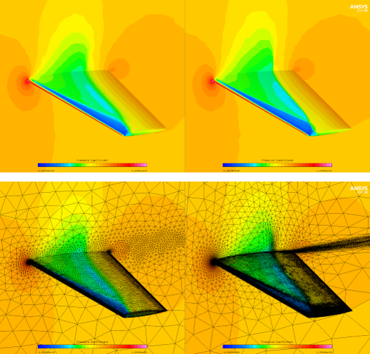
Figure 38.11: Pressure Coefficient Contours and Surface Mesh Along the Wing and Z = 0.75 m Plane - Original Solution (Left) and 2nd Adapted Solution (Right)
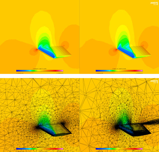
Figure 38.12: 2D Surface Pressure Coefficient Distributions Along the Wing at Z = 0 m (Left) and Z = 0.75 m (Right)
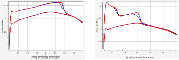
As seen in the figures above, mesh adaptation further refines the mesh at the location of the lambda shock as well as the wake produced by the wing. This extra refinement allows the airflow solver to capture the abrupt pressure drop across the lambda shock (see 2D plot figures). Other wing locations have also been refined, for instance, the leading edge and the wing tip. While in Viewmerical, zoom in near the leading edge of the wing tip. You should obtain a figure similar to the one shown below.
Figure 38.13: Pressure Coefficient Contours and Surface Mesh Along the Leading Edge of the Wing Tip - Original Solution (Left) and 2nd Adapted Solution (Right)
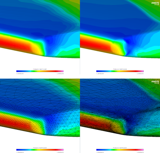
This figure shows how mesh adaptation improved the mesh refinement of the curvature of the leading edge and wing tip. As a result, a more continuous distribution of pressure coefficient along these high velocity gradient locations can be achieved.
Compare mach number contours at the symmetry plane and the Z = 0.75 m plane between the original and the final adapted solution. Enable in the Object panel to only see the contours. You should obtain the following figures.
Figure 38.14: Mach Number Contours at the Symmetry Plane (Top) and the Z = 0.75 m Plane (Bottom) - Original Solution (Left) and 2nd Adapted Solution (Right)
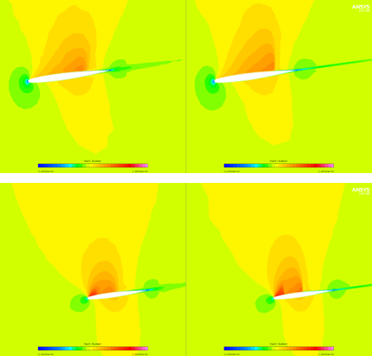
Comparison of mach number contours show that mesh adaptation provides a clear representation of the airflow acceleration around the wing and the sudden deceleration across the shocks. Numerical noise and dissipation have been extensively reduced and the wake has been neatly captured.
Compare turbulent viscosity contours at the symmetry plane and the X = 1.2 m plane between the original and the final adapted solution. Enable and in Object to see the contours in standalone mode and contours with their respective surface mesh. You should obtain the following figures.
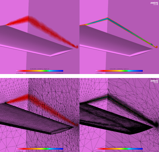
Figure 38.15: Turbulent Viscosity Contours and Surface Mesh Along the Wing, Symmetry Plane and X = 1.2 m Plane - Original Solution (Left) and 2nd Adapted Solution (Right)
Zoom in near the location of the wing tip vortex on the X = 1.2m plane to have a better view of the mesh refinement and the turbulent viscosity at this location. Go back to the Data panel and change Data to to clearly see the orientation of the airflow recirculation at the wake.
Figure 38.16: Turbulent Viscosity at X = 1.2m Plane, Wing Tip Vortex - Original Solution (Left) and 2nd Adapted Solution (Right)
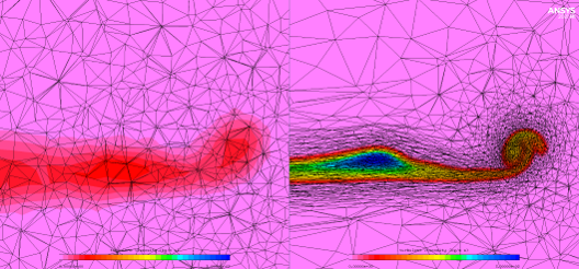
Figure 38.17: Velocity Vectors at X = 1.2m Plane, Wing Tip Vortex - Original Solution (Left) and 2nd Adapted Solution (Right)
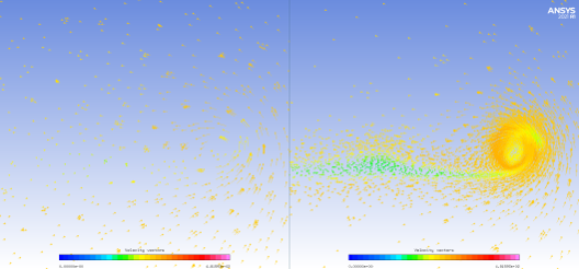
The above figures show the level of mesh refinement that was added during mesh adaptation cycles in order to precisely capture the wake and the wing tip vortex produced by the wing. These phenomena are important to capture especially for high lift configurations or aircraft components that are located in the wake of upstream surfaces.