This tutorial is divided into the following sections:
This tutorial has been divided into two parts. In Part I, you will search for an input angle of attack that results in a target output lift coefficient value. In Part II, you will search for a stall angle of attack that results in a maximum output lift coefficient value. These types of simulations can be useful in external aerodynamics design, as it allows you to investigate a solution, including the drag produced, at a specific or maximum lift performance.
This tutorial, you will search for an input angle of attack that results in a target output lift coefficient value. This type of simulation can be useful in external aerodynamics design, as it allows you to investigate a solution, including the drag produced, at a specific lift performance.
This tutorial is written with the assumption that you have completed the introductory tutorials found in this manual and that you are familiar with the Ansys Fluent outline view and ribbon structure. Some steps in the setup and solution procedure will not be shown explicitly.
Using the ONERAM6 swept wing geometry, and given Freestream Mach and Altitude conditions, a parameter search will be conducted to find
Part I: the angle of attack that produces a requested lift coefficient, and
Part II: the angle of attack that produces the maximum lift coefficient.
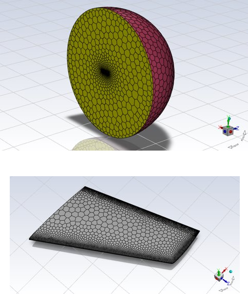
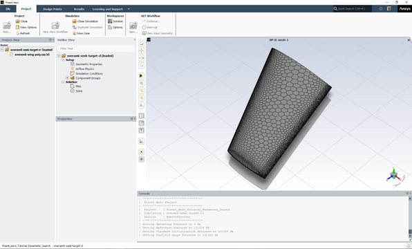
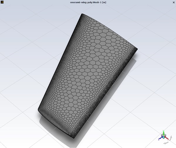
The geometry has been placed inside a hemispherical domain. Fluent Meshing was used to produce a mesh that consists of 114,219 polyhedra cells. This is a very coarse grid. It’s purpose is to ease calculation time and resources while demonstrating these features. Only four layers of prisms were grown off the wing’s wall boundaries to capture the boundary layer. This number is insufficient if the goal is to obtain precise and accurate solutions. This mesh follows the domain type requirements of a Fluent Aero simulation. The limits of the computational domain are defined by a hemispherical boundary that acts as a pressure-far-field, and a flat circular boundary defined as a symmetry plane in the Z direction. For a domain type, the external boundary of the domain should be defined with a pressure-far-field zone, and can optionally include a connected pressure-outlet zone. Refer to Freestream or WindTunnel Domain Type Requirements for more information.
To find the target output value, a secant method is utilized. Multiple calculation cycles are performed. In each cycle, the input parameter is updated and the CFD solution and resulting output parameter is found. The input and output parameters from the previous two cycles are used to define the input parameter for the next cycle. The search will stop if either the search tolerance on the output parameter is reached or the maximum number of cycles is reached.
Finding the maximum output value is a one-dimensional optimization problem. A hybrid search methodology is employed to determine the stall angle of attack, where the lift coefficient reaches its maximum in the angle of attack vs. lift coefficient curve. This hybrid methodology starts with a broad search using a golden section method to identify a narrowed search interval and then uses a quadratic interpolation method to find the maximum lift coefficient and associated angle of attack. The search terminates upon reaching either the combined search tolerance on the input and output parameters or the maximum number of cycles.
The following sections describe the setup and solution steps to find the target lift coefficient for this tutorial:
To prepare for running this tutorial:
Download the fluent_aero_parameter_search.zip file here .
Unzip fluent_aero_parameter_search.zip to your working directory.
The file, oneram6-wing-poly.msh.h5, can be found in the folder.
Launch Fluent 2024 R2 on your computer.
Within the Fluent Launcher, set the Capability Level to Enterprise, then select Aero.
Set Solver Processes to
16under Parallel Processing Options.Click Start.
Alternatively, Fluent Aero can be opened using the aero (on Linux) or aero.bat (on Windows) file inside the fluent/bin/ folder.
Uncheck , , and .
 Project
→ Workspaces → Options
Project
→ Workspaces → Options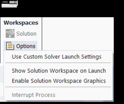
The graphical user interface (GUI) of Fluent Aero is very similar to Fluent, however there are some differences such as:
The ribbon is reduced to only the File, Project, Design Points and View tabs and therefore most actions for setting up your simulation will be performed in the Outline View.
Individual settings are defined in the Properties window which are accessed by left-clicking an item in the Outline View.
Note: Settings in the Properties window are saved as you define them, unlike dialog boxes which require you to click an button.
The console allows for Python scripting and can read Python commands from a journal / script file.
Create a new project file.
File → New
Project...
Enter
Fluent_Aero_Tutorial_Parameter_Searchas the Project file name within the Select File dialog.Select and import the oneram6-wing-poly.msh.h5 input grid.
Project
→ Simulation → New
Aero Workflow
A New Simulation window will appear. Enter the Name of the New Simulation as
oneram6-seek-target-cl, and check to enable . Click .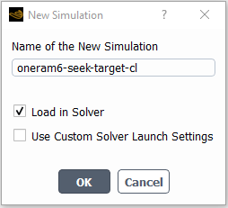
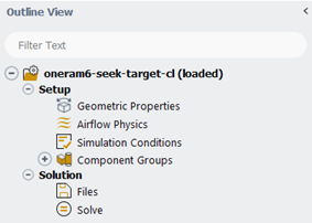
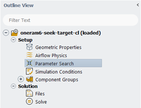
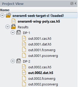
After the .msh.h5 file has been successfully loaded, a new Outline View tree appears under oneram6-seek-target-cl (loaded).
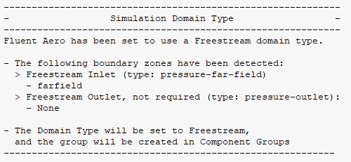
While importing, Fluent Aero will attempt to automatically determine if a Freestream domain type is being used. It will search for the pressure-far-field zone that defines the external boundary of the domain and add it to the Freestream group. Fluent Aero will set the domain type as Freestream, and the following message will be reported in the Console.
The mesh is now displayed in the Graphics Window to the right.
Enable to expose features that are not yet fully supported.
File
→ Preferences... →
Aero → 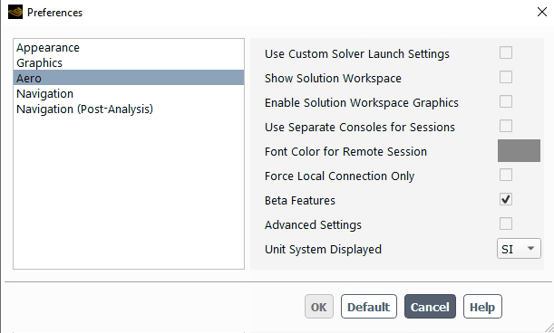
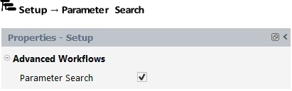
After enabling , toggle on .
 Setup →
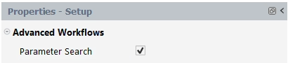
A Parameter Search node now appears in the Outline View.
Define the Geometric Properties of the simulation.
At the top of this new properties window, notice that the Domain Type has been automatically set to .
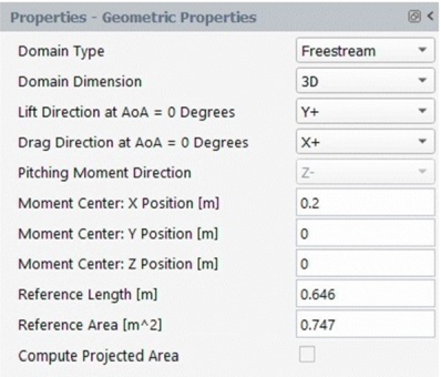
Retain the default selection of for Lift Direction at AoA = 0 degree.
Retain the default selection of for Drag Direction at AoA = 0 degree.
Pitching Moment Direction will automatically be set to .
Set the Moment Center X-, Y- and Z-Position [m] to
0.2,0, and0, respectively.Set the Reference Length [m] to
0.646, which corresponds to the mean chord length.Set the Reference Area [m^2] to
0.747.
Define the Airflow Physics of the simulation.
Setup → Airflow
PhysicsIn the Solver section:
Setup → Airflow
Physics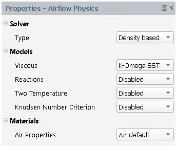
Set Type to .
In the Models section:
Set Viscous to K-Omega SST
Set Corner Flow Correction to Disabled
Set Reactions to .
Set Two Temperature to .
Set Knudsen Number Criterion to .
In the Materials section
Set Air Properties to .
Define the Parameter Search objective of the simulation.
Setup → Parameter
Search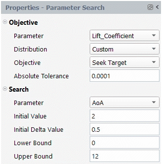
In the Objective section:
Retain the default selection of for Parameter.
Select from the Distribution drop-down list.
Retain the default selection of for Objective.
Retain the value of
0.0001for Absolute Tolerance.
In the Search section:
Retain the default selection of for Parameter.
Retain the value of
2for Initial Value.Retain the value of
0.5for Initial Delta Value.Retain the value of
0for Lower Bound.Retain the value of
12for Upper Bound.
Define the Simulation Conditions of the simulation.
Setup → Simulation
Conditions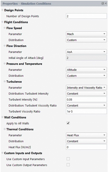
Set the Number of Design Points to
2.In the Flow Speed section:
Retain the default selection of for Parameter.
Select from the Distribution drop-down list.
In the Flow Direction section:
Retain the default selection of for Parameter.
Initial Angle of Attack [deg] will automatically be set to 2.
In the Pressure and Temperature section:
Select from the Parameter drop-down list.
Select from the Distribution drop-down list.
Retain the default selections for the remaining settings.
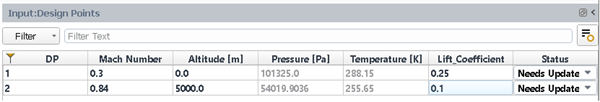
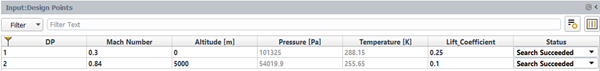
An Input:Design Points table will be created in the graphic window on the right-hand side of the user interface. This table shows all the design points that will be simulated.
Set the Mach Number for DP-1 and DP-2 to
0.3and0.84respectively.Set the Altitude for DP-1 and DP-2 to
0.0and5000.0respectively.Set the Lift_Coefficient for DP-1 and DP-2 to
0.25and0.1respectively.
The initial status of each design point (DP) has been set as .
Define the Solve settings of the simulation.
Solution →
Solve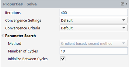
Set the number of Iterations to
400.Select for the Convergence Settings and Convergence Criteria drop-down list.
In the Parameter Search section:
Retain the value of
10for Number of Cycles.Enable Initialize Between Cycles.
Click to launch the design point calculations.
The calculation will start, and the first design point, DP-1, will be simulated. A Convergence window will appear in place of the Graphics window and display the residuals and monitors for DP-1.
Design point DP-1 will continue until the Absolute Tolerance (0.0001) or the maximum Number of Cycles (10) are reached, whichever comes first.
In this example, DP-1 will calculate for up to 10 Number of Cycles, with up to 300 Iterations per cycle. At that point, the conditions will be updated for the next design point and the calculation will resume. This process repeats until all design points are simulated.
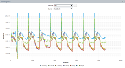
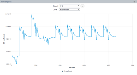
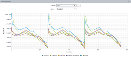
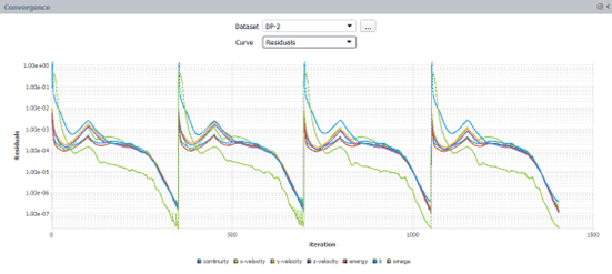
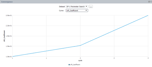
Look at the convergence history of the simulation in the Convergence window located on the right of your screen. Set the Dataset to or and the Curve to , to view the continuity, x- y- z-velocity, energy, and turbulence residuals for the first or second design point. You can left-click a residual curve to show the iteration number and the corresponding residual value.
The standard convergence shows residual changes per iteration. Each angle of attack update is visible by the sharp increase in residuals.
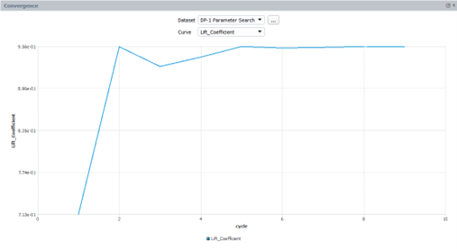
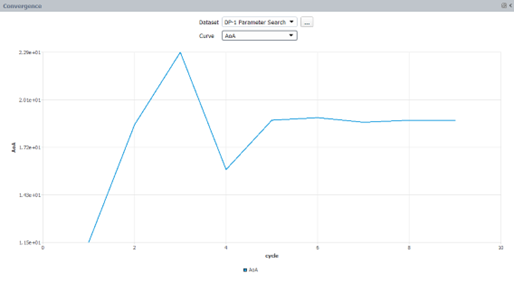
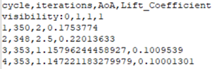
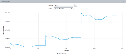
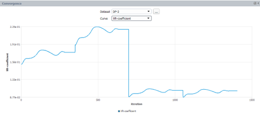
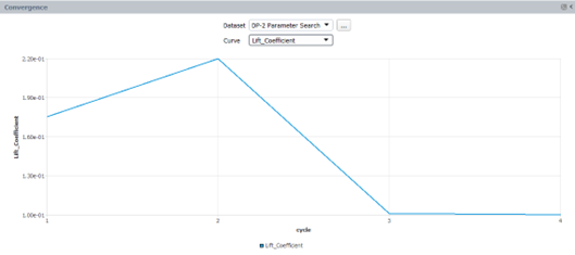
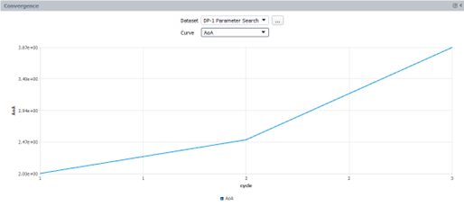
Set the Dataset to or and the Curve to or . This will show the changes to the Objective Parameter () and Search Parameter () per search cycle.
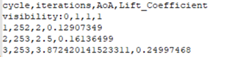
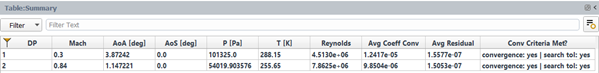
In each Convergence graph, click the last cycle. You will notice that the lift coefficient converges at ~0.249975 at an angle of attack of ~3.8724 degrees after 3 cycles for and to ~0.100013 at an angle of attack of ~1.1472 degrees after 4 cycles for .
Furthermore, the DP-1 folder located in the Project View contains out.0001.psconverg, which houses the text version of what’s plotted within DP-1 Parameter Search.
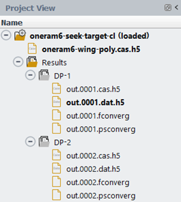
Note: To quickly access and view the text file, right-click the oneram6-seek-target-cl simulation folder, and select . This will open a browser window. Inside the Results folder, find the out.0001.psconverg file, and open it with your preferred text editor.
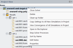
Similarly, the DP-2 folder located in the Project View contains out.0002.psconverg, which houses the text version of what’s plotted in the DP-2 Parameter Search.
After all the design points have been updated, notice that the status of the Input:Design Points table will be set to for all the design points.
A Results node will be displayed in the Outline View tree after the simulation starts. This allows you to quickly post-process design point solutions, by obtaining aerodynamic coefficient plots, creating contour plots of the solution fields, comparing solution fields to experimental data, and more.
In the current tutorial, 2 different Tables will be created automatically in the Graphics window area when the calculation is complete.
Click the Table:Summary and Table:Coefficients tabs at the bottom of the Graphics window to reveal each table.
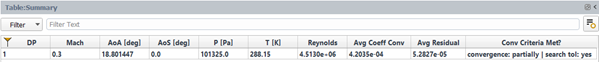
Table:Summary summarizes the final angle of attack in degrees, flight conditions and convergence information for each design point. In the current simulation, all design points have met the convergence criteria and will display convergence: yes | search tol: yes in the Conv Criteria Met? column.
convergence: yes specifies that the convergence cutoff criteria has been met in the final search cycle.
search tol: yes specifies that the search tolerance has been reached.
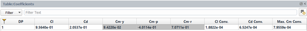
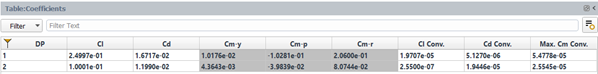
Table:Coefficients contains the lift, drag, yaw moment, pitching moment and rolling moment coefficients. The Cl Conv. and Cd Conv. columns measure the convergence of the lift and drag coefficients. These are used to determine if the convergence criteria are met. The last column shows the maximum value of the convergence of the yaw, pitching and rolling moments.

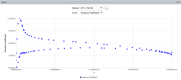
The Plots options can be used to quickly display simple 2D plots of selected design points and solution variables. The Properties - Plots panel will be displayed.
![]() Results → Design Point (DP-1
Loaded) → Plots
Results → Design Point (DP-1
Loaded) → Plots
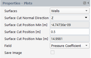
Retain the default selection of for Surfaces.
Retain the default selection of for Surface Cut Normal Direction.
Set Surface Cut Position [m] to
0.5.Retain the default selection of for Field.
Click .
The pressure coefficient on the walls of DP-1 at Z=0.5m will be plotted in the Plots window.
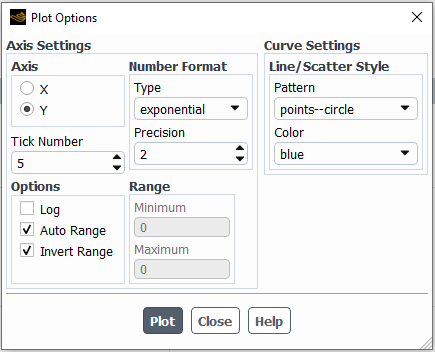
A Plot Options panel will appear after clicking the button. You can use this panel to customize plot settings. Press to apply these settings.
A .csv file will be saved in the Results folder after clicking the button, which is visible within the DP-1/Data folder in the Project View.
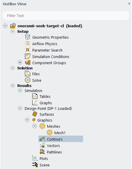
The Contours options can be used to quickly display simple contour plots of selected design points and solution variables.
![]() Results → Design Point (DP-1
Loaded) → Graphics →
Contours
Results → Design Point (DP-1
Loaded) → Graphics →
Contours
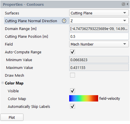
Select from the Surfaces drop-down list.
Select from the Cutting Plane Normal Direction drop-down list.
Set Cutting Plane Position [m] to
0.5.Select from the Field drop-down list.
Click the button.
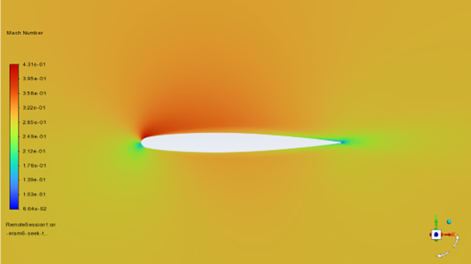
The selected contour will be displayed in the Graphics window.
In the Graphics window, use the mouse to set the view of the contour. Click and rename it to
oneram6-seek-target-cl-view-1. The current contour image can be saved by clicking on the Save Image… button.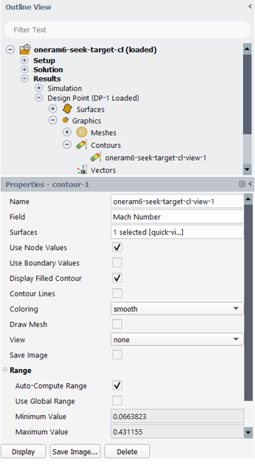
The following sections describe the setup and solution steps to find the maximum lift coefficient for this tutorial:
Open the project created in Part I – Fluent_Aero_Tutorial_Parameter_Search.
In the Project ribbon, select Simulations -> New Aero Workflow and browse to and select the
oneram6-wing-poly.msh.h5file. A New Simulation window will appear. Enter the Name of the New Simulation as oneram6-seek-maximum-cl and check Load in Solver.Enable Beta Features to expose features that are not yet fully supported.
File
→ Preferences → Aero → Beta
FeaturesAfter enabling Beta Features, toggle on Parameter Search
Set the Geometric Properties and Airflow Physics as in Part I – Seek Target Lift Coefficient.
Define the Parameter Search objective of the simulation.
Setup →
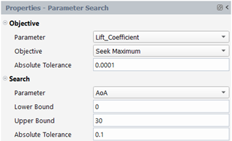
In the Objective section:
Retain the default selection of Lift_Coefficient for Parameter.
Select Seek Maximum from the Objective drop-down list.
Retain the value of
0.0001for Absolute Tolerance.
In the Search section:
Retain the default selection of AoA for Parameter.
Retain the value of
0for Lower Bound.Retain the value of
30for Upper Bound.Retain the value of
0.1for Tolerance.
Define the Simulation Conditions of the simulation.
Setup →
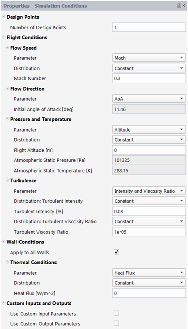
Set the Number of Design Points to 1.
In the Flow Speed section:
Retain the default selection of Mach for Parameter.
Retain the default selection of Constant for Distribution.
Set the Mach Number to 0.3
In the Flow Direction section:
Retain the default selection of AoA for Parameter.
Initial Angle of Attack [degrees] will automatically be set to 11.46.
In the Pressure and Temperature section:
Select Altitude from the Parameter drop-down list.
Retain the default selection of Constant for Distribution.
Set the Flight Altitude [m] to 0.
Retain the default selections for the remaining settings.
Define the Solve settings of the simulation.
Setup →
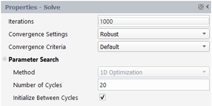
Select Robust from the Convergence Settings drop-down list.
Set the number of Iterations to 1000.
In the Parameter Search section:
Retain the value of 20 for Number of Cycles.
Retain the toggle on for Initialize Between Cycles.
Click Update to launch the design point calculations.
The calculation will start, and the design point, DP-1, will be simulated. A Convergence window will appear in place of the Graphics window and display the residuals and monitors for DP-1.
Design point DP-1 will continue until the Absolute Tolerances (Lift_Coefficient = 0.0001 and AoA = 0.1) or the maximum Number of Cycles (20) are reached, whichever comes first.
In this example, DP-1 will calculate for up to 20 Number of Cycles, with up to 1000 Iterations per cycle. At that point, the conditions will be updated for the next design point, if any, and the calculation will resume. This process repeats until all design points are simulated.
Look at the convergence history of the simulation in the Convergence window located on the right of your screen. Set the Dataset to DP-1 and the Curve to Residuals, to view the continuity, x- y- z-velocity, energy, and turbulence residuals for the current design point. You can left-click a residual curve to show the iteration number and the corresponding residual value.
The standard convergence shows residual changes per iteration. Each angle of attack update is visible by the sharp increase in residuals.
Set the Dataset to DP-1 Parameter Search and the Curve to AoA or Lift_Coefficient. This will show the changes to the Objective Parameter (Lift_Coefficient) and Search Parameter (AoA) per search cycle.
In the Convergence graph, click the last cycle. You will notice that the lift coefficient converges at ~0.9564 at an angle of attack of ~18.8014 degrees after 9 cycles for DP-1 Parameter Search.
Furthermore, the DP-1 folder located in the Project View contains
out.0001.psconverg, which houses the text version of what’s plotted within DP-1 Parameter Search.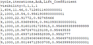
After the current design point has been updated, notice that the status of the Input:Design Points table will be set to Search Succeeded.
A Results node will be displayed in the Outline View tree after the simulation starts. This allows you to quickly post-process design point solutions, by obtaining aerodynamic coefficient plots, creating contour plots of the solution fields, comparing solution fields to experimental data, and more, as demonstrated in section Post-processing
In the current tutorial, 2 different Tables will be created automatically in the Graphics window area when the calculation is complete.
Click the Table:Summary and Table:Coefficients tabs at the bottom of the Graphics window to reveal each table.
Table:Summary summarizes the final angle of attack in degrees, flight conditions and convergence information for each design point. In the current simulation, the design point has met the convergence criteria and will display convergence: partially | search tol: yes in the Conv Criteria Met? column.
convergence: partially specifies that the default convergence cutoff criteria have been partially met in the final search cycle.
Note: The Lift_Coefficient must either converge or exhibit stable oscillations in all cycles to accurately determine the maximum Lift_Coefficient. If oscillations occur, the average values of the periodic oscillations are used for 2.5D meshes, and instantaneous values at the end of the cycles are used for 3D meshes. Additionally, convergence can be enhanced by utilizing a high-quality mesh and/or by switching Convergence Settings to Custom and adjusting Solution parameters
Search tol: yes specifies that the search tolerance has been reached.
Table:Coefficients contains the lift, drag, yaw moment, pitching moment and rolling moment coefficients. The Cl Conv. and Cd Conv. columns measure the convergence of the lift and drag coefficients. These are used to determine if the convergence criteria are met. The last column shows the maximum value of the convergence of the yaw, pitching and rolling moments.