17.5. Modeling Hypersonic Flows Using the Two-Temperature Model

When using the density-based solver, a two-temperature model is available for simulating the thermal non-equilibrium phenomena in hypersonic flows. It models the energy relaxation process in the flow and provides a better prediction of the flow fields than the one-temperature model.

Note: Additional feature license is required to enable the use of this model. Please contact your Ansys representative to check for the availability of the license increment.

For more information, see The Two-Temperature Model for Hypersonic Flows in the Fluent Theory Guide.

17.5.1. Using the Two-Temperature Model

To use the two-temperature model, perform the following steps:

Select Density-Based from the Type list in the General task page.
Setup → General
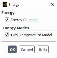
Enable the Energy Equation along with the Two-Temperature Model option.
Setup → Models → Energy
Figure 17.3: The Energy Dialog Box
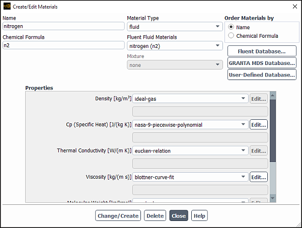
Define the fluid in the Create/Edit Materials dialog box. Note that when the Two-Temperature Model is enabled, the material properties have appropriate models selected for the Density, Specific Heat (Cp), Thermal Conductivity, and Viscosity. For details about these models, see The Two-Temperature Model for Hypersonic Flows in the Fluent Theory Guide.
The available methods for Specific Heat (Cp) are nasa-9-piecewise-polynomial (default, see Inputs for NASA-9-Piecewise-Polynomial Functions) and Boltzmann-kinetic-theory.
Setup → Materials → Create/Edit...
Figure 17.4: The Create/Edit Materials Dialog Box

If you do not copy a material from the Fluent database, be sure to do the following:
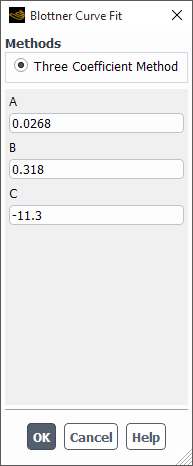
- Click the Edit... button for the Viscosity, and enter appropriate values for the fields in the Blottner Curve Fit dialog box. For details, see Blottner/Eucken/Constant Lewis in the Fluent Theory Guide.
  Figure 17.5: The Blottner Curve Fit Dialog Box
- If the species is atomic or diatomic, select constant for the Characteristic Vibrational Temperature and enter an appropriate value.
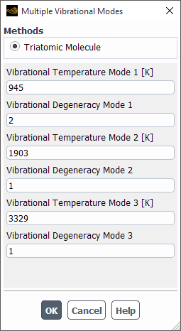
- If the species is triatomic, select vibrational-modes for the Characteristic Vibrational Temperature input the vibrational temperature and degeneracy for each mode in the Multiple Vibrational Modes dialog box.
  Figure 17.6: The Multiple Vibrational Modes Dialog Box
Note: If your simulation is modeling the flow of a mixture, it is recommended that you define materials for each of the individual molecules and then use the species transport model to create a mixture material (as described in later steps). For example, if modeling air, define a material for nitrogen () and oxygen ().
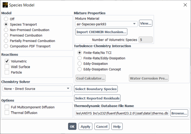
If modeling the flow of a mixture, enable the Species Transport model in the Species Model dialog box.
Setup → Models → Species
1. Import a mixture suitable for your simulation. For detailed information about the available mixtures, see Modeling Non-Equilibrium Gas Dissociation Using Finite Rate Chemistry.
2. Select Volumetric for Reactions.
3. Select either None - Direct Source (recommended) or Stiff Chemistry Solver for Chemistry Solver.
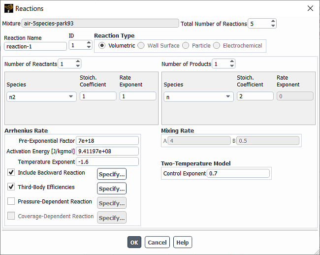
  Figure 17.7: Species Model Dialog Box with Settings for Two-Temperature Model
4. In the Reactions dialog box (accessed by clicking Edit... next to Reaction on the Create/Edit Materials dialog box for the mixture), you can specify the Control Exponent for each reaction.
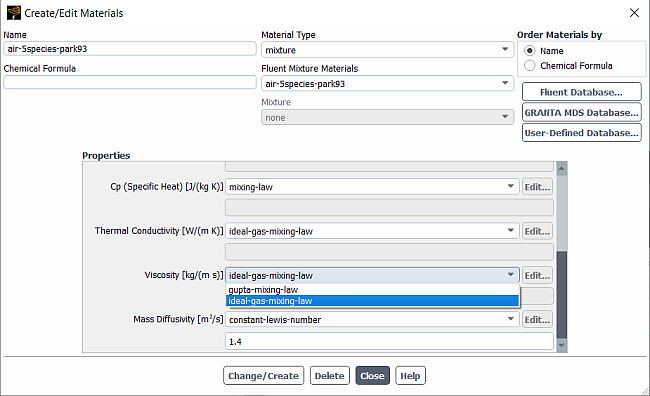
  Figure 17.8: Reactions Dialog Box with Settings for Two-Temperature Model
5. In the Create/Edit Materials dialog box, when the material type is a mixture, the available methods for Thermal Conductivity and Viscosity are ideal-gas-mixing-law (default) and gupta-mixing-law. The available methods for Mass Diffusivity are constant-lewis-number (default, with a constant of 1.4) and gupta-mixing-law.
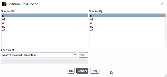
  Figure 17.9: Create/Edit Materials Dialog Box for Mixture
6. When gupta-mixing-law is selected, the collision cross-section coefficients are provided for the air-2species-nitrogen, air-5species-park93, air-11species-park93, and air-11species-gupta mixtures. After clicking Change/Create, you can examine the coefficients by editing the cross-section-multicomponent method.
Figure 17.10: The Collision Cross Section Dialog Box for air-5species-park93 Mixture

For more details on the Two-Temperature model with species, see Finite-Rate Chemistry with the Two-Temperature Model in the Fluent Theory Guide and The Two-Temperature Model for Hypersonic Flows in the Fluent Theory Guide.
Note: The following are capabilities and limitations for the Two-Temperature and Species models:
- If using the Stiff Chemistry solver, Direct integration is supported.
- If using the Stiff Chemistry solver, ISAT, Dynamic Mechanism Reduction, or Chemistry Agglomeration are not supported.
- The None - Direct Source chemistry solver is recommended.
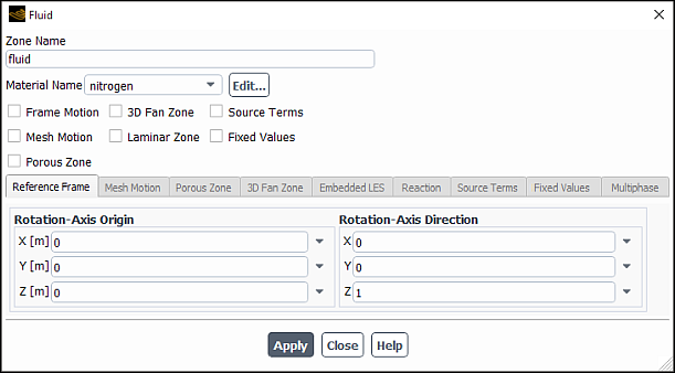
For the cell zone, select the fluid for the Material Name in the Fluid dialog box.
Setup → Cell Zone Conditions → Fluid
Figure 17.11: The Fluid Dialog Box
If modeling the flow of a mixture, specify the fractions of the molecules in the Species tab of the boundary condition dialog boxes.
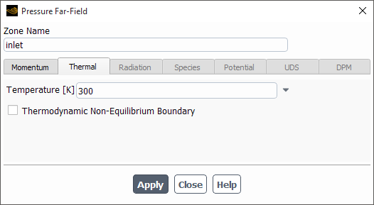
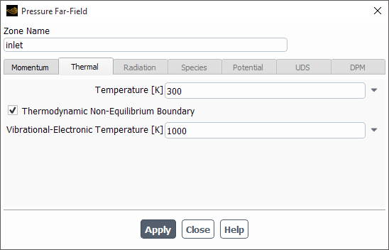
When defining the Boundary Conditions, select an appropriate boundary condition type. On the boundary, local thermodynamic equilibrium is assumed and the temperature can be specified in the thermal dialog box.
Figure 17.12: Pressure Far-Field Dialog Box
For Pressure Far-Field and Velocity-Inlet boundary conditions, you can set the vibrational-electronic temperature different from the translational-rotational temperature by clicking the Thermodynamic Non-Equilibrium Boundary box and specifying the Vibrational-Electronic Temperature.
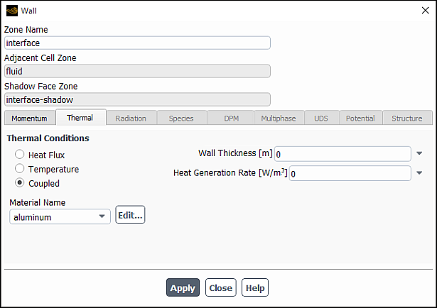
Figure 17.13: Pressure Far-Field Dialog Box with Non-Equilibrium Boundary Option
For two-sided (coupled) walls, you can select Coupled for Thermal Conditions. Local thermodynamic equilibrium is assumed on the interior and exterior sides of the wall.
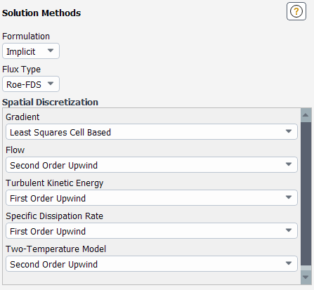
Figure 17.14: Two-sided Wall Dialog Box with Coupled Option
When defining the Solution Methods task page, select an appropriate spatial discretization scheme from the Two-Temperature Model drop-down list.
Solution → Methods
Figure 17.15: The Solution Methods Task Page
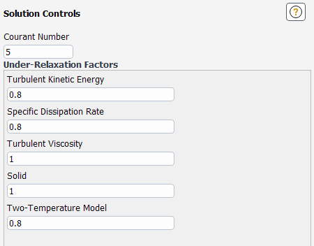
When defining the Solution Controls task page, enter an appropriate under-relaxation factor for the Two Temperature Model field.
Solution → Controls
Figure 17.16: The Solution Controls Task Page

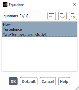
Note that during the course of your simulations, you have the option of disabling the calculation of the vibrational-electronic energy equations by deselecting the Two Temperature Model item in the Equations dialog box prior to running the calculation.
Solution → Controls → Equations...
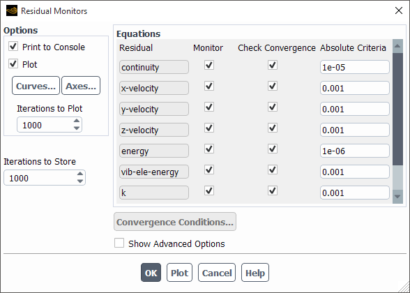
Figure 17.17: The Equations Dialog Box
When setting up the residual monitors, note that you have the option of monitoring and checking convergence based on the vibrational-electronic energy (vib-ele-energy).
Solution → Monitors → Residual
Figure 17.18: The Residual Monitors Dialog Box
After running the calculations, you can postprocess the following field variables under the Two Temperature Model... category:
- Translational-Rotational Temperature
  This is in Equation 5–23 in the Fluent Theory Guide. It is equivalent to the Static Temperature field under the Temperature... category.
- Vibrational-Electronic Temperature
  This is in Equation 5–23 in the Fluent Theory Guide.
- Internal Energy
  This the sum of the translational-rotational energy and vibrational-electronic energy and is the same as the Internal Energy field under the Temperature... category.
- Translational-Rotational Energy
  This is the sum of the translational and rotational energy ( and in Equation 5–38 in the Fluent Theory Guide).
- Vibrational-Electronic Energy
  This is the sum of the vibrational and electronic energy ( and in Equation 5–38 in the Fluent Theory Guide).
- Translational-Rotational over Vibrational-Electronic Temperature
  This is the ratio of translational-rotational temperature over vibrational-electronic temperature.
- Vibrational-Electronic Conductivity
  This is the vibrational-electronic conductivity of the mixture.
- Vibrational-Electronic Specific Heat
  This is the vibrational-electronic specific heat of the mixture.
- Mass-Averaged Relaxation Time
  This is the mass-averaged translational-vibrational relaxation time.
- Frozen Sound Speed
  This is defined as where is the translational-rotational heat capacity ratio.
- Dissociation Vibration Source
  This is the vibrational-electronic energy change due to chemical reactions ( in Equation 5–28 in the Fluent Theory Guide).
Note: The definition of the Total Temperature under the Temperature... category is adjusted to include the contribution from the vibrational-electronic energy. Local thermal equilibrium is assumed, and the total temperature is computed from the total enthalpy.