


The following are a few examples that demonstrate why or where you may want to use an expression and how you would do so for these situations.
The following example shows you how to define a parabolic inlet profile for laminar pipe flow, as shown in Figure 5.9: Contours of Velocity - Parabolic Inflow. In this example, the pipe is centered in the X and Z directions and the pipe axis is aligned to the Y-direction.
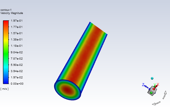
The expression for defining the parabolic inflow shown in Figure 5.9: Contours of Velocity - Parabolic Inflow is Equation 5–1,
 | (5–1) |
Where  is the velocity at the axis,
  is the radius of the pipe, and
  is the local radial coordinate.
To fully define this example:
Create a named expression for the maximum velocity called umax.
 Setup → Named
Expressions
Setup → Named
Expressions  New...
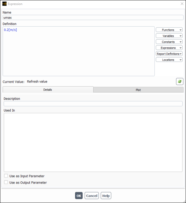
Enter umax for the Name.
Enter 0.2 [m/s] for the Definition and click .
Create an expression for the radius of the pipe.
Open the Expressions dialog box by right-clicking Named Expressions in the outline view tree and selecting New....
Enter Radius for the Name.
Enter sqrt(Area(["in"])/PI) for the Definition. "in" is the name of the inlet boundary. PI is the expression constant for Pi.
Click to create the named expression.
Create an expression for the local radial profile.
Open the Expressions dialog box and enter radius for the Name.
Enter sqrt(x**2+z**2) for the Definition. This expression uses the square root mathematical expression operator.
Click to create the named expression.
Create an expression for the inlet velocity profile. This expression combines the other expressions you created.
Open the Expressions dialog box and enter uprofile for the Name.
Enter umax*(1- (radius/Radius)**2) for the Definition. You can use the Expressions drop-down to the right of the Definition box to add named expressions to your expression definition as an alternative to typing the names manually.
Click to create the named expression.
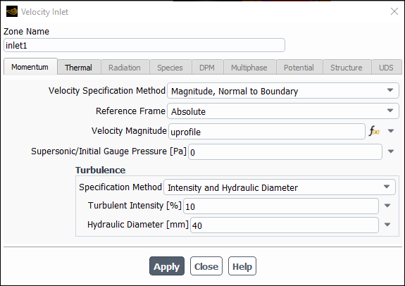
Assign uprofile to the velocity inlet.
Setup → Boundary
Conditions → Inlet
→ in Edit...
You can group the boundary conditions by type to organize the boundaries and reduce the size of the list. This can be accomplished by right-clicking Boundary Conditions in the tree and selecting Group By> Zone Type.
Select expression from the drop-down to the right of Velocity Magnitude.
Enter uprofile in the Velocity Magnitude field and click .
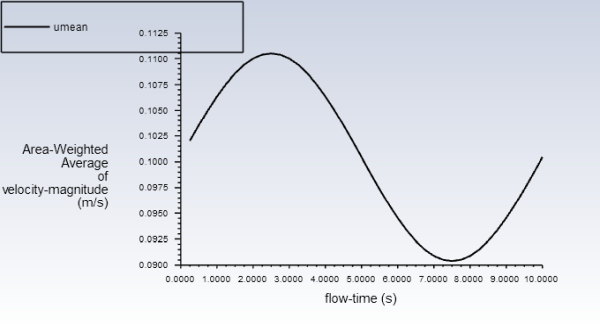
The following example shows you how to define a parabolic inlet profile for laminar pipe flow that varies over time (a sine function with a period of 10 seconds). The velocity profile in this example is the same as for Parabolic Inflow Profile except it is for a transient simulation because the velocity varies over time. Figure 5.10: Parabolic Inflow Velocity Over Time plots the area weighted average of the velocity magnitude over 10 seconds.
To create an expression for this time-varied velocity profile:
Define all of the named expressions as described in Parabolic Inflow Profile.
Create an expression for omega.
Setup → Named
Expressions New...
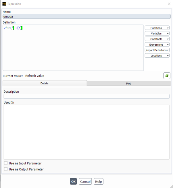
Enter omega for the Name.
Enter 2*PI / (10[s]) for the Definition and click .
Create an expression for the velocity profile that varies over time.
Open the Expressions dialog box and enter uprofile_transient for the Name.
Enter uprofile*(sin(omega*Time)*0.1 + 1) for the Definition and click .
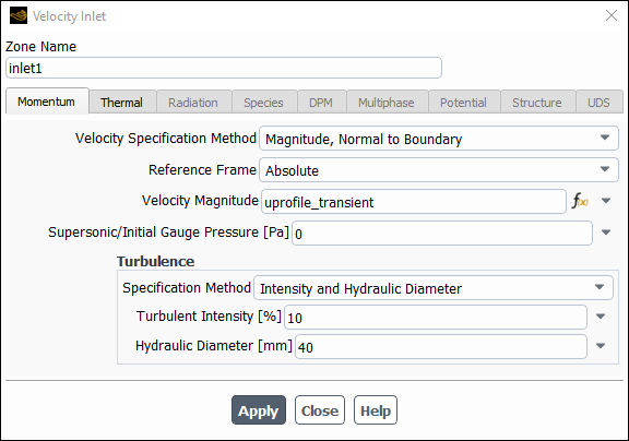
Assign uprofile_transient to the velocity inlet.
Setup → Boundary
Conditions → Inlet
→ in Edit...
You can group the boundary conditions by type to organize the boundaries and reduce the size of the list. This can be accomplished by right-clicking Boundary Conditions in the tree and selecting Group By> Zone Type.
Select expression from the drop-down to the right of Velocity Magnitude.
Enter uprofile_transient in the Velocity Magnitude field and click .
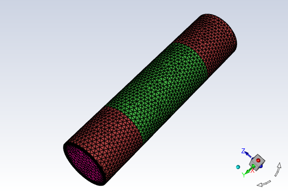
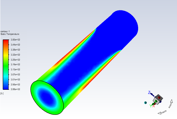
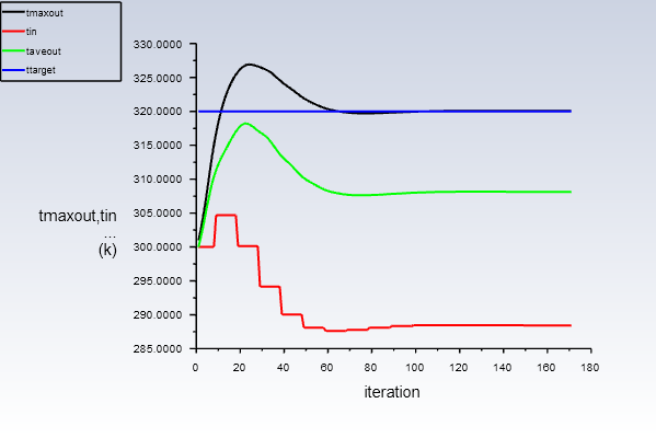
The following example shows you how to drive the maximum temperature at the outlet to a target temperature by varying the inlet temperature. For this scenario, a pipe with laminar flow has a part of the wall that is heated to 350 Kelvin and a target outlet temperature of 320 Kelvin (Figure 5.11: Pipe Geometry Colored by ID (Heated Wall is Green) shows the portion of the wall that is heated). A controller turns on every 10th iteration (steady-state case) and adjusts the inlet temperature according to Equation 5–2. In the other iterations, the controller leaves the temperature unchanged. This is achieved by using the conditional statement given in Equation 5–3. Figure 5.12: Contours of Temperature (outlet is closest) shows the developed temperature profile for this case.
 | (5–2) |
 | (5–3) |
 is the formula used to adjust the inlet temperature,
  is the current inlet temperature,
  is the target temperature for the outlet, which is set to 320 Kelvin,
 is the maximum temperature at the outlet, and
  is a relaxation factor.
The following steps show how to create the expressions used in this example:
Create a named expression for the initial temperature, called TStart.
Setup → Named
Expressions New...
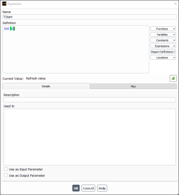
Enter TStart for the Name.
Enter 300 [K] for the Definition and click .
Create an expression for the target temperature for the outlet, called TTarget, and set it equal to 320 [K]. Use the same process that you used to create TStart.
Create an expression for the maximum temperature that occurs at the outlet, called TMaxOut. In this expression you will be using a function to determine the maximum temperature.
Click the Functions drop-down and select Reduction → Maximum.
Enter StaticTemperature for the first field of the function and ["out"] for the location. The total expression should appear as Maximum(StaticTemperature, ["out"]).
Create an expression for the current inlet temperature, called TInCurrent, and set it equal to Average(StaticTemperature, ["in"], Weight=None). Use a similar process to what you used to create TMaxOut, but with selecting the Average function instead.
Create an expression for the relaxation factor, called relax, and set it equal to 0.9.
Create an expression for adjusting the inlet temperature, called TAdjust, and set it equal to TInCurrent + (TTarget - TMaxOut)*relax.
Create an expression for the inlet temperature, which will be called TIn, and set it equal to IF(iter<5, TStart, IF(mod(iter+1, 10)==0, TAdjust, TInCurrent)). Use a similar process to what you used to create TMaxOut, but with selecting the IF conditional function instead.
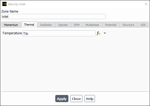
Assign TIn to the inlet.
Setup → Boundary
Conditions → Inlet
→ in Edit...
Select expression from the drop-down to the right of Temperature.
Enter TIn in the Temperature field and click .
The following example shows you how to setup to use dot(),
vector(), moment(), and
force() expression operations in Ansys Fluent. Six expressions are
defined: AOA, dragForce, flowDir, liftForce, moment, and totalForce.
To begin, define the angle of attack expression as an input parameter.
Open the Expression dialog box.
Setup → Named
Expressions New...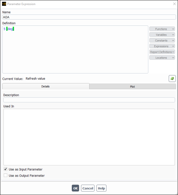
Note that the dialog box appears as Parameter Expression because the setup is already completed and Use as Input Parameter is enabled.
Enter
AOAas the Name.Enter
5[deg]in the Definition field.Enable Use as Input Parameter.
Click to create the angle of attack input parameter expression.
Define the flow direction.
Open the Expression dialog box.
Setup → Named
Expressions New...Enter
flowDiras the Name.Enter
vector(cos(AOA), sin(AOA), 0.0)in the Definition field.Note: You select expressions that you have already defined, such as AOA from the Expressions drop-down list on the right-hand side of the dialog box.
Click to create the expression for the flow direction.
Define the total force.
Open the Expression dialog box.
Setup → Named
Expressions New...Enter
totalForceas the Name.Enter
Force(['wall-top', 'wall-bottom'])in the Definition field.Click to create the expression for the total force.
Define the moment about the centroid of the airfoil.
Open the Expression dialog box.
Setup → Named
Expressions New...Enter
momentas the Name.Enter
Moment(Centroid(['fluid-16'], ['wall-top',
              'wall-bottom']).mag
in the Definition field.Enable Use as Output Parameter to use the moment as an output parameter.
Click to create the expression for the total force.
Define the lift force normal to the flow.
Open the Expression dialog box.
Setup → Named
Expressions New...Enter
liftForceas the Name.Enter
dot(totalForce, vector(-flowDir.y, flowdir.x, 0))in the Definition field.Note: You select expressions that you have already defined, such as totalForce from the Expressions drop-down list on the right-hand side of the dialog box.
Enable Use as Output Parameter to use the lift force as an output parameter.
Click to create the expression for the lift force.
Define the drag force.
Open the Expression dialog box.
Setup → Named
Expressions New...Enter
dragForceas the Name.Enter
dot(totalForce, flowDir)in the Definition field.Note: You select expressions that you have already defined, such as totalForce from the Expressions drop-down list on the right-hand side of the dialog box.
Enable Use as Output Parameter to use the drag force as an output parameter.
Click to create the expression for the total force.
Now that these expressions are defined, you can include them in expression report definitions for monitoring and judging convergence.