


This chapter provides basic instructions to install the magnetohydrodynamics (MHD) module and solve MHD problems in Ansys Fluent. It assumes that you are already familiar with standard Ansys Fluent features, including the user-defined function procedures described in the Fluent Customization Manual. Guidelines For Using the Ansys Fluent MHD Model also outlines the general procedure for using the MHD model. This chapter describes the following:
The MHD module is provided as an add-on module with the standard Ansys Fluent licensed
software. The module is installed in a directory called
addons/mhd in your installation area. The MHD module
consists of a UDF library and a pre-compiled Scheme library, which must be loaded
and activated before calculations can be performed.
The MHD module can be loaded into Ansys Fluent only when a valid Ansys Fluent case file has been set or read.
There are two different ways in which you can load the MHD module into Ansys Fluent:
Through the ribbon
In the Physics ribbon tab, click (Models group), and select MHD Model....
 Physics →
Models → More
→ MHD Model
Physics →
Models → More
→ MHD ModelOnce the MHD module is loaded into Ansys Fluent, the MHD Model dialog box opens with the Enable MHD option automatically selected (see Figure 33.2: The MHD Model Dialog Box).
Through the text user interface (TUI)
The text command to load the module is
define→models→addon-module.A list of Ansys Fluent add-on modules is displayed:
> /define/models/addon-module
Fluent  Addon Modules:
     0. None
     1. MHD Model
     2. Fiber Model
     3. Fuel Cell and Electrolysis Model
     4. SOFC Model with Unresolved Electrolyte
     5. Population Balance Model
     6. Adjoint Solver
     7. Single Potential Battery Module
     8. MSMD Battery Model
     9. PEM Fuel Cell Model
Enter Module Number: [0] 1
Select the MHD model by entering the module number 1.
Once the MHD module is loaded into Ansys Fluent, you can enable the MHD model as described in Enabling the MHD Model.
During the loading process a Scheme library containing the graphical and text user interface, and a UDF library containing a set of user defined functions are loaded into Ansys Fluent. A message Addon Module: mhd...loaded! is displayed at the end of the loading process.
The basic set up of the MHD model is performed automatically when the MHD module is loaded successfully. The set up includes:
Selecting the default MHD method
Allocating the required number of user-defined scalars and memory locations naming of:
User-defined scalars and memory locations
All UDF Hooks for MHD initialization and adjustment
MHD equation flux and unsteady terms
Source terms for the MHD equations
Additional source terms for the fluid momentum and energy equations
Default MHD boundary conditions for external and internal boundaries
A default set of model parameters
DPM related functions are also set, if the DPM option has been selected in the Ansys Fluent case set up.
The MHD module set up is saved with the Ansys Fluent case file. The module is loaded automatically when the case file is subsequently read into Ansys Fluent. Note that in the saved case file, the MHD module is saved with the absolute path. Therefore, if the locations of the MHD module installation or the saved case file are changed, Ansys Fluent will not be able to load the module when the case file is subsequently read.
To unload the previously saved MHD module library, open the UDF Library Manager dialog box
![]() Parameters & Customization
→ User Defined Functions
Parameters & Customization
→ User Defined Functions
![]() Manage...
Manage...
and reload the module as described above. Note that the previously saved MHD model setup and parameters are preserved.
The settings related to the MHD model are specified in the MHD Model dialog box, which can be accessed either via the tree:
![]() Setup → Models
→ MHD Model
Setup → Models
→ MHD Model ![]() Edit...
Edit...
or using the text command:
define →
models → mhd-model
Both the MHD Model dialog box and TUI commands are designed for the following tasks:
Enable/disable the MHD model.
Select the MHD method.
Apply an external magnetic field.
Set boundary conditions.
Set solution control parameters.
Operations of these tasks through the MHD Model dialog box are described in the following sections. The set of MHD text commands are listed in Magnetohydrodynamics Text Commands .
For more information, see the following sections:
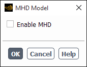
If the MHD model is not yet enabled after the MHD module is loaded, you can enable it by selecting Enable MHD in the MHD Model dialog box, shown in Figure 33.1: Enabling the MHD Model Dialog Box. The dialog box expands to its full size when the model is enabled, as shown in Figure 33.2: The MHD Model Dialog Box.
The method used for MHD calculation can be selected under MHD Method in the MHD Model dialog box. The two methods, Magnetic Induction and Electrical Potential, are described in Magnetic Induction Method and Electric Potential Method,
For the Magnetic Induction method, 2 or 3 user-defined scalars are allocated for the solution of the induced magnetic field in 2D or 3D cases. The scalars are listed as B_x, B_y and B_z representing the Cartesian components of the induced magnetic field vector. The unit for the scalar is Tesla.
For the Electrical Potential method, 1 user-defined scalar is solved for the
electric potential field. The scalar is listed as  and has the unit of Volt.
Table 33.1: User-Defined Scalars in MHD Model lists the user-defined scalars used by the two methods.
Table 33.1: User-Defined Scalars in MHD Model
| Method | Scalar | Name | Unit | Description |
|---|---|---|---|---|
| Induction | Scalar-0 | B_x | Tesla | X component of induced magnetic field
( ) ) |
| Scalar-1 | B_y | Tesla | Y component of induced magnetic field
( ) ) | |
| Scalar-2 (3-D) | B_z | Tesla | Z component of induced magnetic field
( ) ) | |
| Potential | Scalar-0 | Phi | Volt | Electric potential ( ) ) |
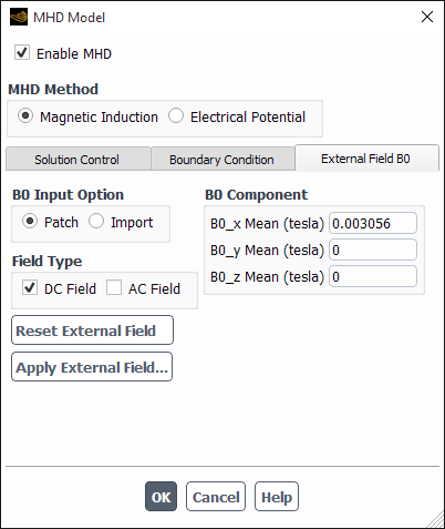
Application of an external magnetic field to the computation domain is done under the External Field B0 tab in the MHD Model dialog box, as shown in Figure 33.3: The MHD Model Dialog Box for Patching an External Magnetic Field. Two B0 Input Options are available for setting up the external magnetic field. One option is to Patch the computational domain with a constant (DC Field) and/or varying (AC Field) type. The other option is to Import the field data from a magnetic data file that you provide.
With the Patch option enabled, the AC field can be expressed as a function of time (specified by Frequency), and space (specified by wavelength, propagation direction and initial phase offset). The space components are set under the B0 Component, as in Figure 33.3: The MHD Model Dialog Box for Patching an External Magnetic Field.
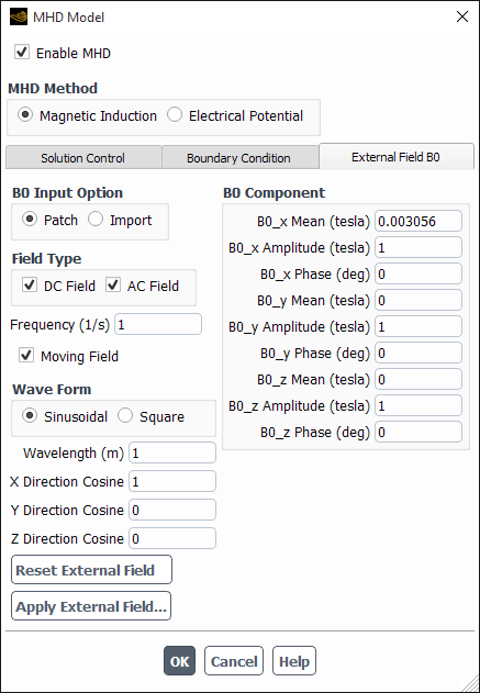
You can also specify a Moving Field with a wave form that is either a sinusoidal or a square wave function (Figure 33.4: The MHD Model Dialog Box for Specifying a Moving Field). Definitions for the sinusoidal and square wave forms of patched magnetic fields are provided in Definitions of the Magnetic Field.
Selecting Import under the B0 Input Option in the MHD Model dialog box, as seen in Figure 33.5: The MHD Model Dialog Box for Importing an External Magnetic Field, will result in the import of magnetic field data. The data filename can be entered in the B0 Data File Name field, or selected from your computer file system using the Browse... button. Magnetic data can also be generated using a third-party program such as MAGNA. The required format of the magnetic field data file is given in External Magnetic Field Data Format.
When using the Import option, the B0 Data Media is either set to Non-Conducting or Conducting, depending on the assumptions used in generating the magnetic field data. (These choices correspond to “Case 1” and “Case 2”, respectively, as discussed in Magnetic Induction Method.)
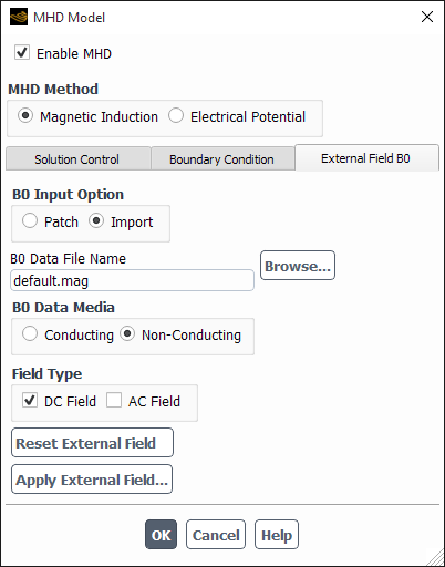
The Field Type is determined by the field data from the data file. The choice of either the DC Field or the AC Field option in the dialog box is irrelevant if the import data is either DC or AC. However, selection of both options indicates that data of both field types are to be imported from the data file, and superimposed together to provide the final external field data. Make sure that the data file contains two sections for the required data. See External Magnetic Field Data Format for details on data file with two data sections.
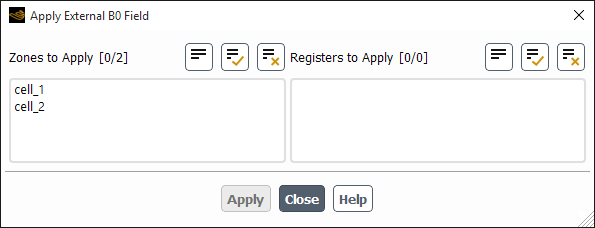
The Apply External Field... button opens the Apply External B0 Field dialog box as shown in Figure 33.6: Apply External B0 Field Dialog Box. To apply the external field data to zones or regions in the computational domain, select the zone names or register names of marked regions from the dialog box and click the Apply button.
The Reset External Field button sets the external magnetic field variable to zero.
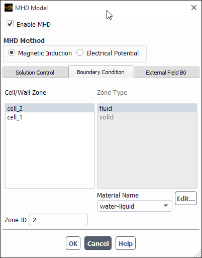
Boundary conditions related to MHD calculations are set under the Boundary Condition tab in the MHD Model dialog box. Boundary conditions can be set to cell zones and wall boundaries.
Note: Note that all boundary conditions used by the MHD model must be set in the Boundary Condition tab of the MHD Model dialog box. Customized boundary conditions of any form, such as parameters and expressions, are not supported.
For cell zones, only the associated material can be changed and its properties modified. Figure 33.7: Cell Boundary Condition Setup shows the dialog box for cell zone boundary condition setup. The cell zone material can be selected from the Material Name drop-down list.
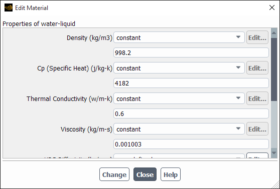
Note that the materials available in the list are set in the general Ansys Fluent case set up. Refer to the Ansys Fluent User Guide for details on adding materials to an Ansys Fluent case. The properties of the selected material can be modified in the Boundary Condition tab by clicking to the right of the material name. This opens the Edit Material dialog box, as shown in Figure 33.8: Editing Material Properties within Boundary Condition Setup. The material properties that may be modified include the electrical conductivity and magnetic permeability. The material electrical conductivity can be set as constant, a function of temperature in forms of piecewise-linear, piecewise-polynomial or polynomial, or as a user-defined function. The material magnetic permeability can only be set as a constant.
For wall boundaries, the boundary condition can be set as an Insulating Wall, Conducting Wall, Coupled Wall or Thin Wall (Magnetic Induction method only). The dialog box for wall boundary condition set up is shown in Figure 33.9: Wall Boundary Condition Setup.
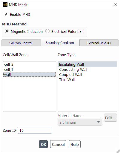
The insulating wall is used for boundaries where there is no electric current going through the boundary.
The conducting wall is used for boundaries that are perfect conductors.
The coupled wall should be used for wall boundaries between solid/solid or solid/fluid zones where the MHD equations are solved.
(Magnetic Induction method only) The thin wall type boundary can be used for external wall that has a finite electrical conductivity.
For conducting walls and thin wall boundaries, the wall material can be selected from the Material Name drop-down list, and its properties modified through the Edit Material dialog box. A wall thickness must be specified for thin wall type boundaries.
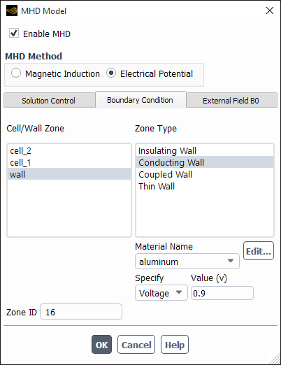
If the Electric Potential method is selected, the conducting wall boundary is specified by either of Voltage or Current Density at the boundary, as shown in Figure 33.10: Conducting Wall Boundary Conditions in Electrical Potential Method.
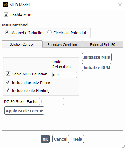
Under the Solution Control tab in the MHD Model dialog box, Figure 33.11: Solution Control Tab in the MHD Model Dialog Box, a number of parameters can be set that control the solution process in an MHD calculation. The MHD model can be initialized using the Initialize MHD button. When the DPM model is enabled in the Ansys Fluent case set up, the related variables used in the MHD model can be initialized using the Initialize DPM button.
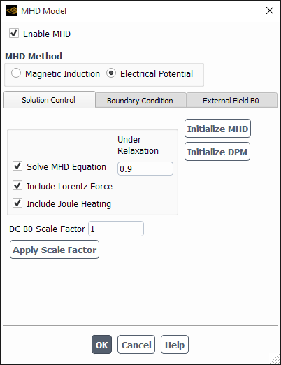
You have the option to enable or disable the Solve MHD Equation. When the Solve MHD Equation is enabled, you have the choice to Include Lorentz Force and/or Include Joule Heating in the solution of flow momentum and energy equations. The under-relaxation factor for the MHD equations can also be set.
The strength of the imposed external magnetic field can be adjusted by specifying and applying scale factors to the external DC and/or AC magnetic field data.
The following sections describe the solution and postprocessing steps for the MHD model:
Initialization of the MHD model involves setting the externally-imposed magnetic field and initializing all MHD related user-defined scalars and memory variables.
When an Ansys Fluent case is initialized, all user-defined scalar and memory variables are set to zero. The external magnetic field data is set from the External Field B0 tab in the MHD Model dialog box. The Initialize MHD button under the Solution Control tab can be used to initialize the model during an Ansys Fluent solution process. It is used when MHD effects are added to a fully or partially solved flow field, or when the model parameters are changed during an MHD calculation. It only clears the scalar variables and most of the memory locations used in the MHD model, the memory variables for the external magnetic field data are preserved.
It is often an effective strategy to begin your MHD calculations using a
previously-converged flow field solution. With this approach, the induction
equations themselves are generally easy to converge. The under-relaxation
factors for these equations can be set to 0.8  0.9, although for very strong magnetic fields, smaller values
may be needed. For the electric potential equation, the convergence is generally
slow. However, the under-relaxation value for this equation should not be set to
1. As additional source terms are added to the momentum and energy equations,
the under-relaxation factors for these equations should generally be reduced to
improve the rate of convergence. In case of convergence difficulties, another
helpful strategy is to use the B0 Scale Factor in the
Solution Control tab (Figure 33.2: The MHD Model Dialog Box). This will gradually increase the MHD
effect to its actual magnitude through a series of restarts. When the strength
of the externally imposed magnetic field is strong, it is advisable to start the
calculation with a reduced strength external field by applying a small scale
factor. When the calculation is approaching convergence the scale factor can be
increased gradually until the required external field strength is
reached.
0.9, although for very strong magnetic fields, smaller values
may be needed. For the electric potential equation, the convergence is generally
slow. However, the under-relaxation value for this equation should not be set to
1. As additional source terms are added to the momentum and energy equations,
the under-relaxation factors for these equations should generally be reduced to
improve the rate of convergence. In case of convergence difficulties, another
helpful strategy is to use the B0 Scale Factor in the
Solution Control tab (Figure 33.2: The MHD Model Dialog Box). This will gradually increase the MHD
effect to its actual magnitude through a series of restarts. When the strength
of the externally imposed magnetic field is strong, it is advisable to start the
calculation with a reduced strength external field by applying a small scale
factor. When the calculation is approaching convergence the scale factor can be
increased gradually until the required external field strength is
reached.
You can use the standard postprocessing facilities of Ansys Fluent to display the MHD calculation results.
Contours of MHD variables can be displayed using
![]() Results →
Graphics → Contours
Results →
Graphics → Contours
![]() Edit...
Edit...
The MHD variables can be selected from the variable list.
Vectors of MHD variables, such as the magnetic field vector and current density vector, can be displayed using
![]() Results →
Graphics → Vectors
Results →
Graphics → Vectors
![]() Edit...
Edit...
The vector fields of the MHD variables are listed in the Vectors of drop-down list in the Vectors dialog box. Table 33.2: MHD Vectors lists the MHD related vector fields.
Table 33.2: MHD Vectors
| Name | Unit | Description |
|---|---|---|
Induced-  -Field -Field | Tesla | Induced magnetic field vector |
External-  -Field -Field | Tesla | Applied external magnetic field vector |
Current-Density 
|

| Induced current density field vector |
Electric-Field 
| V/m | Electric field density vector |
Lorentz-Force 
|

| Lorentz force vector |
Note:
For field variables that are stored in UDM, use the corresponding variables for postprocessing. Postprocessing the UDM itself is not recommended.
For reviewing simulation results in CFD-Post for cases involving UDM or UDS, export the solution data as CFD-Post-compatible file (.cdat) in Fluent and then load this file into CFD-Post.
Many MHD applications involve the simultaneous use of other advanced Ansys Fluent capabilities such as solidification, free surface modeling with the volume of fluid (VOF) approach, DPM, Eulerian multiphase, and so on. You should consult the latest Ansys Fluent documentation for the limitations that apply to those features. In addition, you should be aware of the following limitations of the MHD capability.
As explained in Modeling Magnetohydrodynamics, the MHD module assumes a sufficiently conductive fluid so that the charge density and displacement current terms in Maxwell’s equations can be neglected. For marginally conductive fluids, this assumption may not be valid. More information about this simplification is available in the bibliography.
For electromagnetic material properties, only constant isotropic models are available. Multiphase volume fractions are not dependent on temperature, species concentration, or field strength. However, sufficiently strong magnetic fields can cause the constant-permeability assumption to become invalid.
You must specify the applied magnetic field directly. The alternative specification of an imposed electrical current is not supported.
In the case of alternating-current (AC) magnetic fields, the capability has been designed for relatively low frequencies; explicit temporal resolution of each cycle is required. Although not a fundamental limitation, the computational expense of simulating high-frequency effects may become excessive due to small required time step size. Time-averaging methods to incorporate high-frequency MHD effects have not been implemented.