Turbulent flows are significantly affected by the presence of walls. Obviously, the mean velocity field is affected through the no-slip condition that has to be satisfied at the wall. However, the turbulence is also changed by the presence of the wall in non-trivial ways. Very close to the wall, viscous damping reduces the tangential velocity fluctuations, while kinematic blocking reduces the normal fluctuations. Toward the outer part of the near-wall region, however, the turbulence is rapidly augmented by the production of turbulence kinetic energy due to the large gradients in mean velocity.

The near-wall modeling significantly impacts the fidelity of numerical solutions, inasmuch as walls are the main source of mean vorticity and turbulence. After all, it is in the near-wall region that the solution variables have large gradients, and the momentum and other scalar transports occur most vigorously. Therefore, accurate representation of the flow in the near-wall region determines successful predictions of wall-bounded turbulent flows.

Numerous experiments have shown that the near-wall region can be largely subdivided into three layers. In the innermost layer, called the "viscous sublayer", the flow is almost laminar, and the (molecular) viscosity plays a dominant role in momentum and heat or mass transfer. In the outer layer, called the fully-turbulent layer, turbulence plays a major role. Finally, there is an interim region between the viscous sublayer and the fully turbulent layer where the effects of molecular viscosity and turbulence are equally important. Figure 4.15: Subdivisions of the Near-Wall Region illustrates these subdivisions of the near-wall region, plotted in semi-log coordinates.

Figure 4.15: Subdivisions of the Near-Wall Region

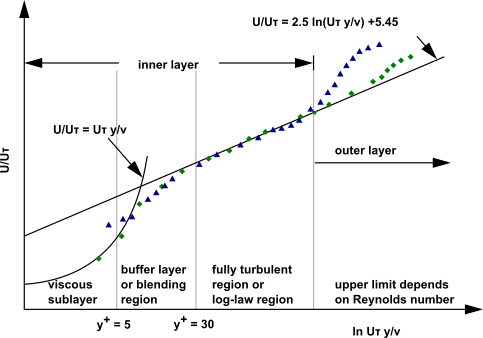
In Figure 4.15: Subdivisions of the Near-Wall Region, , where is the friction velocity, defined as .

Wall Functions vs. Near-Wall Model

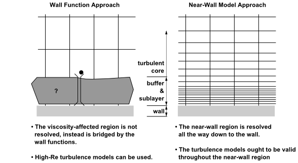
Traditionally, there are two approaches to modeling the near-wall region. In one approach, the viscosity-affected inner region (viscous sublayer and buffer layer) is not resolved. Instead, semi-empirical formulas called "wall functions" are used to bridge the viscosity-affected region between the wall and the fully-turbulent region. The use of wall functions obviates the need to modify the turbulence models to account for the presence of the wall.

In another approach, the turbulence models are modified to enable the viscosity-affected region to be resolved with a mesh all the way to the wall, including the viscous sublayer. For the purposes of discussion, this will be termed the "near-wall modeling" approach. These two approaches are depicted schematically in Figure 4.16: Near-Wall Treatments in Ansys Fluent.

Figure 4.16: Near-Wall Treatments in Ansys Fluent

The main shortcoming of all wall functions (except the scalable wall function) is that the numerical results deteriorate under refinement of the grid in the wall normal direction. values less than 15 will gradually result in unbounded errors in wall shear stress and wall heat transfer. While this was the industrial standard some years ago, Ansys Fluent has taken steps to offer more advanced wall formulations, which allow a consistent mesh refinement without a deterioration of the results. Such -independent formulations are the default for all -equation-based turbulence models. For the -equation-based models, the Menter-Lechner and Enhanced Wall Treatment (EWT) serve the same purpose. A -insensitive wall treatment is also the default for the Spalart-Allmaras model and allows you to run this model independent of the near-wall resolution.

High quality numerical results for the wall boundary layer will only be obtained if the overall resolution of the boundary layer is sufficient. This requirement is actually more important than achieving certain values. The minimum number of cells to cover a boundary layer accurately is around 10, but values of 20 are desirable. It should also be noted that an improvement of boundary layer resolution can often be achieved with moderate increase in numerical effort, as it requires only a mesh refinement in the wall-normal direction. The associated increase in accuracy is typically well worth the additional computing costs. For unstructured meshes, it is recommended that you generate prism layers near the wall with 10–20 or more layers for an accurate prediction of the wall boundary layers. The thickness of the prism layer should be designed to ensure that around 15 or more nodes are actually covering the boundary layer. This can be checked after a solution is obtained, by looking at the turbulent viscosity, which has a maximum in the middle of the boundary layer – this maximum gives an indication of the thickness of the boundary layer (twice the location of the maximum gives the boundary layer edge). It is essential that the prism layer is thicker than the boundary layer as otherwise there is a danger that the prism layer confines the growth of the boundary layer.

Recommendations: