Chapter 11: Using the Frozen Rotor Method

This tutorial is divided into the following sections:

11.1. Introduction

In this tutorial, you will setup a general fluid flow simulation to evaluate the performance of a centrifugal pump with a vaneless volute using the Frozen Rotor method.

This tutorial demonstrates how to do the following:

Set up a No Pitch-Scale interface using the turbo model.
Describe wall motion and other boundary conditions.
Specify appropriate solver settings.
Add and monitor expressions.
Calculate expressions and display contours.

11.2. Prerequisites

This tutorial is written with the assumption that you have completed the introductory tutorials found in this manual and that you are familiar with the Ansys Fluent outline view and ribbon structure. Some steps in the setup and solution procedure will not be shown explicitly.

11.3. Problem Description

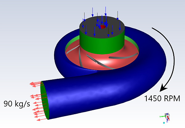
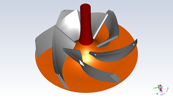
The problem to be considered is the modeling of a centrifugal pump with a volute as shown in Figure 11.1: Case Geometry. The pump impeller has 5 blades and rotates at a velocity of 1450 RPM. The mass flow rate at the volute outlet is known to be 90 kg/s. A gauge total pressure of 0 pa is used at the inlet. The simulation will be performed to determine the head generated by the pump, representing the overall pressure increase of the fluid.

Figure 11.1: Case Geometry

11.4. Setup and Solution

The following sections describe the setup and solution steps for this tutorial:

11.4.1. Preparation

To prepare for running this tutorial:

Download the pump_volute.zip file here .
Unzip pump_volute.zip to your working directory.
The mesh file pump_volute.msh.h5 can be found in the folder.
Use the Fluent Launcher to start Ansys Fluent.
Select Solution in the top-left selection list to start Fluent in Solution Mode.
Select 3D under Dimension.
Enable Double Precision under Options.
Set Solver Processes to 4 under Parallel (Local Machine).

11.4.2. Mesh

Read the mesh file pump_volute.msh.h5.
File → Read → Mesh...
As Fluent reads the mesh file, it will report the progress in the console.
In the Mesh group box of the Domain ribbon tab, set the units for angular-velocity.
Domain → Mesh → Units...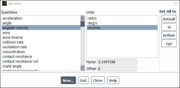
1. Select angular-velocity under Quantities.
2. Select rev/min under Units.
3. Close the Set Units dialog box.

11.4.3. Models

Enable the - SST turbulence model.
Physics → Models → Viscous...
1. Retain the default k-omega SST turbulence model.
2. Click OK.
Compared to other two-equation models, the - SST turbulence model effectively predicts flow separation in turbomachinery, allowing for accurate evaluation of pump performance.

11.4.4. Materials

Add water to the list of materials.
Physics → Materials → Create/Edit...
1. Click Fluent Database... to open the Fluent Database Materials dialog box.
2. Scroll down and select water-liquid (h2o <l>) from the list of materials.
3. Select Copy.
4. Close the Fluent Database Materials dialog box and the Create/Edit Materials dialog box.
water-liquid appears under Materials > Fluid in the tree view.

11.4.5. Cell Zone Conditions

Set the cell zone conditions for the impeller.
Setup → Cell Zone Conditions → Fluid → impeller (fluid, id=36) Edit...
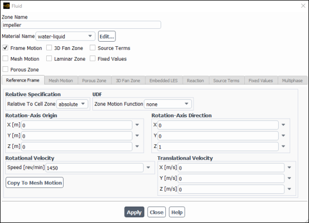
1. Set the Material Name to water-liquid.
2. Select Frame Motion.
3. Ensure values of (0, 0, 1) for X, Y, and Z in the Rotation-Axis Direction group box.
  The impeller will rotate relative to the absolute frame. By default, the correct rotation is set (about the z-axis).
4. For Rotational Velocity → Speed (rpm), specify 1450.
5. Click Apply and close the Fluid dialog box.
Set the cell zone conditions for the volute.
Setup → Cell Zone Conditions → Fluid → volute (fluid, id=2) 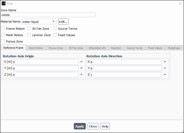Edit...
1. Set the Material Name to water-liquid.
  The volute is stationary in the absolute frame so no motion is required.
2. Ensure values of (0, 0, 1) for X, Y, and Z in the Rotation-Axis Direction group box.
3. Click Apply and close the Fluid dialog box.

11.4.6. Boundary Conditions

Set the boundary conditions for impeller-hub.

Setup → Boundary Conditions → Wall → impeller-hub (wall, id=3) Edit...

Tab	Setting	Value
Momentum	Wall Motion	Moving Wall
Momentum	Motion	Rotational

By default, the rotating wall is specified with a velocity of 0 relative to the impeller fluid zone.

Click Apply and close the Wall dialog box.

Set the boundary conditions for inblock-shroud (wall, id=14).

Setup → Boundary Conditions → Wall → inblock-shroud Edit...

Tab	Setting	Value
Momentum	Wall Motion	Moving Wall
	Motion	Absolute
	Motion	Rotational

The inblock shroud wall is stationary (velocity equal to 0) relative to the absolute reference frame.

Click Apply and close the Wall dialog box.

Set the boundary conditions for the inlet.

Setup → Boundary Conditions → Inlet → inlet (pressure-inlet, id=15) Edit...

Tab	Setting	Value
Momentum	Supersonic/Initial Gauge Pressure	-100 (pascal)

Click Apply and close the Pressure Inlet dialog box.

Set the boundary conditions for the outlet.

The outlet has been automatically set as an inlet by Fluent. You must first change this boundary condition to a mass flow outlet.

Setup → Boundary Conditions → Inlet → mass-flow-inlet-11 (mass-flow-inlet, id=11) Type → mass-flow-outlet

Setup → Boundary Conditions → Outlet → mass-flow-outlet-11 (mass-flow-outlet, id=11) Edit...

Rename the boundary zone to outlet.

Tab	Setting	Value
Momentum	Mass Flow Rate	90 (kg/s)

Click Apply and close the Mass-Flow Outlet dialog box.

11.4.7. Turbomachinery Models

Enable the Turbo Models.
Domain → Turbomachinery and select Turbo Models.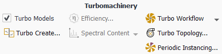
Create the turbo interfaces.
Domain → Turbomachinery → Turbo Create...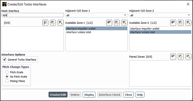

The Frozen Rotor method will be modeled using the No Pitch-Scale (NPS) interface which allows for connecting a 360-degree interface to another 360-degree interface.
1. Enter nps for Mesh Interface.
2. Select interface-impeller-outlet from the Available Zone-1 selection list.
3. Select interface-volute-inlet from the Available Zone-2 selection list.
4. Enable the General Turbo Interface option in the Interface Options group box.
5. Select No Pitch-Scale in the Pitch-Change Types group box under General Turbo Interface.
6. Click Create/Edit and close the Create/Edit Turbo Interfaces dialog box.
Check the mesh.
Domain → Mesh → Check → Perform Mesh Check
Fluent will perform various checks on the mesh and will report the progress in the console. Make sure that the reported minimum volume is a positive number.
Note that if this step is performed before creating the mesh interface, the check will fail because Fluent will detect that the interface is missing.

11.4.8. Solution

Specify the solution methods.
Solution → Solution → Methods...
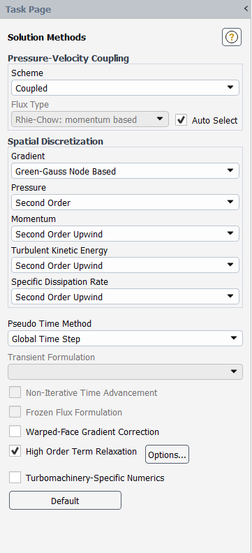
1. Select Green-Gauss Node Based from the Gradient drop-down list in the Spatial Discretization group box.
2. Enable the High Order Term Relaxation option.
3. Retain the default selections.
Create a surface report definition for total pressure at the outlet.
Solution → Reports → Definitions → New → Surface Report → Mass-Weighted Average...
1. Enter p-out for the Name of the surface report definition.
2. Select Pressure... → Total Pressure from the Field Variable drop-down lists.
3. Select Outlet from the Surfaces selection list.
  This automatically selects all the outlet boundary conditions that have been specified.
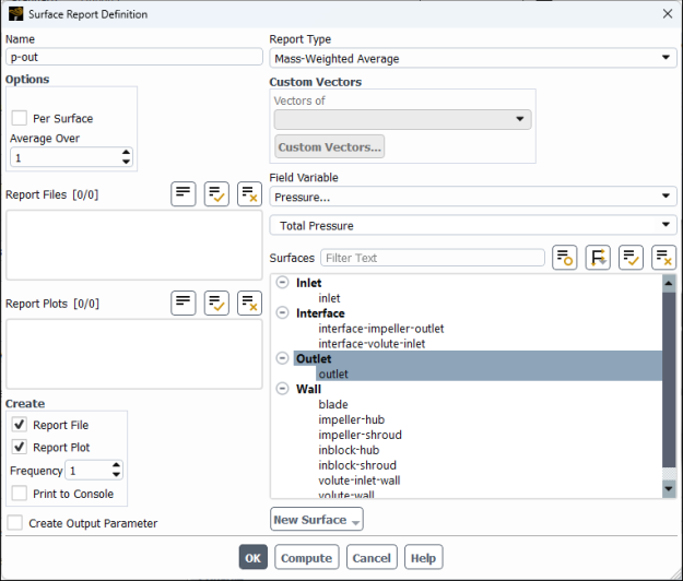
4. Click OK to save the surface report definition settings and close the Surface Report Definition dialog box.
Create a surface report definition for total pressure at the inlet.
Solution → Reports → Definitions → New → Surface Report → Mass-Weighted Average...
1. Enter p-in for the Name of the surface report definition.
2. Select Pressure... and Total Pressure from the Field Variable drop-down lists.
3. Select Inlet from the Surfaces selection list.
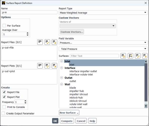
4. Click OK to save the surface report definition settings and close the Surface Report Definition dialog box.
Create a surface report definition for blade pressure.
Solution → Reports → Definitions → New → Surface Report → Integral...
1. Enter p-blade for the Name of the surface report definition.
2. Select Pressure... and Static Pressure from the Field Variable drop-down lists.
3. Select blade from the Surfaces selection list.
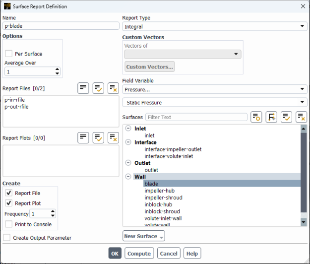
4. Click OK to save the surface report definition settings and close the Surface Report Definition dialog box.
Create an expression for pump head.
Solution → Reports → Definitions → New → Expression...
1. Enter the expression ({p-out} - {p-in}) / (998.2[kg/m^3] * 9.81[m/s^2]).
  You can insert the report definitions you previously created using the Report Definitions drop-down.
  The expression uses 998.2 as the density of water [kg/m^3] and 9.81 as the acceleration of the fluid due to gravity [m/s^2].
2. Enter head for Name.
3. Select Report Plot
4. Select Print to Console
5. Click OK to save the expression and close the Expression Report Definition dialog box.
Initialize the solution.
Solution → Initialization
1. Click More Settings... to open the Hybrid Initialization dialog box.
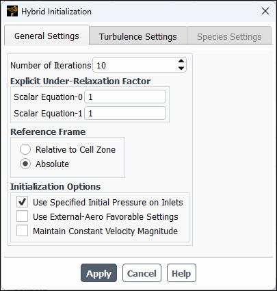
2. Select Absolute under Reference Frame.
3. Select Use Specified Initial Pressure on Inlets under Initialization Options.
4. Click Apply and close the Hybrid Initialization dialog box.
5. Click Initialize to initialize the solution.
Save the case file (pump_volute.cas.h5).
File → Write → Case...
Start the calculation.
Solution → Run Calculation → Run Calculation...
1. Enter 10 for Time Scale Factor.
2. Enter 200 for Number of Iterations.
3. Click Calculate.
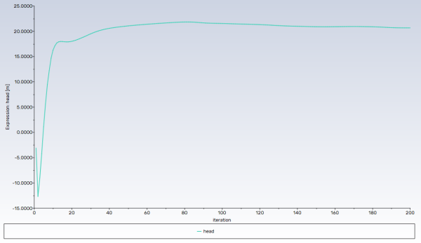
You can monitor the progression of the residuals and the pump head during the run.
Figure 11.2: Convergence History of the Pump Head
Save the case and data files (pump_volute.cas.h5 and pump-volute.dat.h5).
File → Write → Case & Data...

11.4.9. Postprocessing

Determine the head generated from the pump
Solution → Reports → Definitions → Edit...
1. Select head and p-blade from the Report Definitions selection list.
2. Click Compute.
  The head generated by the pump and pressure integral on the blade are printed to the console and are approximately 20.7 [m] and 5650 [pascal m^2], respectively.
Create a contour showing the flow uniformity at the outlet.
Results → Graphics → Contours → New...
1. Enter contour-vel-out for Contour Name.
2. Ensure that the Filled option is enabled in the Options group box.
3. Disable the Global Range option in the Options group box.
4. Select Velocity... and Velocity Magnitude from the Contours of drop-down lists.
5. Deselect all surfaces and select Outlet from the Surfaces selection list.
6. Select Draw Mesh.
7. On the Mesh Display dialog box that opens, deselect all surfaces and select the Wall surface type from the Surfaces selection list.
8. Click Display and close the Mesh Display dialog box.
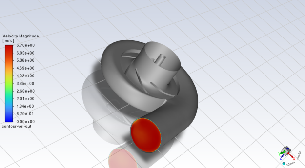
9. Click Save/Display and close the Contours dialog box. Orient the view as shown in Figure 11.3: Contours of Velocity Magnitude at the Outlet.
  This gives an idea of how the fluid is exiting the volute.
  Figure 11.3: Contours of Velocity Magnitude at the Outlet
Create a contour showing cross-sectional pressure.
Results → Graphics → Contours → New...
1. Enter contour-pressure-wall for Contour Name
2. Ensure that the Filled option is enabled in the Options group box.
3. Disable the Global Range option in the Options group box.
4. Select Banded in the Coloring group box.
5. Ensure Pressure... and Static Pressure are selected from the Contours of drop-down lists.
6. Select Wall from the Surfaces selection list.
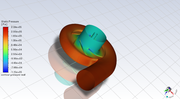
7. Click Save/Display and close the Contours dialog box.
  The increasing pressure in the flow domain can be seen in the contour plot.
  Figure 11.4: Contours of Static Pressure on the Walls
Create filled contours of static pressure.
Results → Graphics → Contours → New...
1. Enter contour-pressure for Contour Name
2. Ensure that the Filled option is enabled in the Options group box.
3. Select Banded in the Coloring group box.
4. Ensure Pressure... and Static Pressure are selected from the Contours of drop-down lists.
5. Select blade, impeller-hub and inblock-hub from the Surfaces selection list.
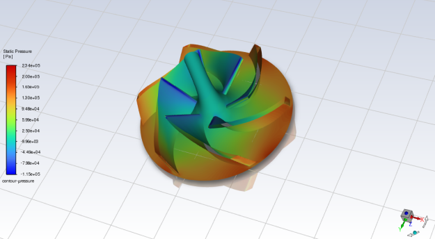
6. Click Save/Display and close the Contours dialog box.
  Pressure distribution in the flow domain is plotted in graphics window.
  Figure 11.5: Contours of Static Pressure
Save the case file (pump_volute.cas.h5).
File → Write → Case...

11.5. Summary

In this tutorial you completed a fluid flow simulation to evaluate the performance of a pump and volute. You created a custom expression to determine the head generated by the pump. While a steady-state simulation was used to model the pump performance using the frozen rotor method, this simulation can be converted to a transient rotor stator simulation by following these steps:

Switch the solver to transient
In the impeller cell zone, change the motion from Frame Motion to Mesh Motion by clicking on Copy to Mesh Motion
In the Run Calculation panel, enter Time Step

You can watch a video of this case being set up, solved, and postprocessed at:

11.6. Further Improvements

This tutorial guides you through the steps to reach a basic solution. You can explore what effect varying certain parameters, such as impeller speed and outlet flow, have on the performance of the pump.