Chapter 16: Modeling Species Transport and Gaseous Combustion

This tutorial is divided into the following sections:

16.1. Introduction

This tutorial examines the mixing of chemical species and the combustion of a gaseous fuel.

A cylindrical combustor burning methane () in air is studied using the eddy-dissipation model in Ansys Fluent.

This tutorial demonstrates how to do the following:

Enable physical models, select material properties, and define boundary conditions for a turbulent flow with chemical species mixing and reaction.
Initiate and solve the combustion simulation using the pressure-based solver.
Examine the reacting flow results using graphics.
Predict thermal and prompt NOx production.
Use custom field functions to compute NO parts per million.

16.2. Prerequisites

This tutorial is written with the assumption that you have completed the introductory tutorials found in this manual and that you are familiar with the Ansys Fluent outline view and ribbon structure. Some steps in the setup and solution procedure will not be shown explicitly.

To learn more about chemical reaction modeling, see the Fluent User's Guide and the Fluent Theory Guide. Otherwise, no previous experience with chemical reaction or combustion modeling is assumed.

16.3. Problem Description

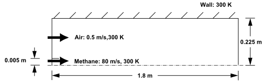
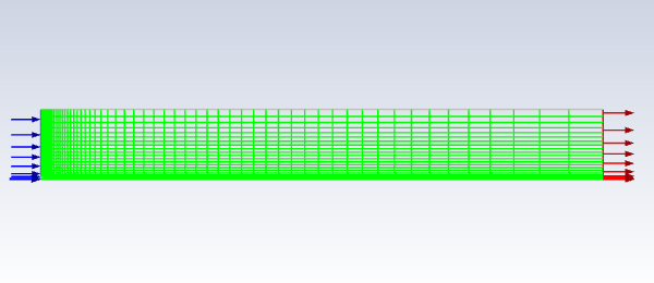
The cylindrical combustor considered in this tutorial is shown in Figure 16.1: Combustion of Methane Gas in a Turbulent Diffusion Flame Furnace. The flame considered is a turbulent diffusion flame. A small nozzle in the center of the combustor introduces methane at 80 . Ambient air enters the combustor coaxially at 0.5 . The overall equivalence ratio is approximately 0.76 (approximately 28 excess air). The high-speed methane jet initially expands with little interference from the outer wall, and entrains and mixes with the low-speed air. The Reynolds number based on the methane jet diameter is approximately .

Figure 16.1: Combustion of Methane Gas in a Turbulent Diffusion Flame Furnace

16.4. Background

In this tutorial, you will use the generalized eddy-dissipation model to analyze the methane-air combustion system. The combustion will be modeled using a global one-step reaction mechanism, assuming complete conversion of the fuel to and . The reaction equation is

(16–1)

This reaction will be defined in terms of stoichiometric coefficients, formation enthalpies, and parameters that control the reaction rate. The reaction rate will be determined assuming that turbulent mixing is the rate-limiting process, with the turbulence-chemistry interaction modeled using the eddy-dissipation model.

16.5. Setup and Solution

The following sections describe the setup and solution steps for this tutorial:

16.5.1. Preparation

To prepare for running this tutorial:

Download the species_transport.zip file here .
Unzip species_transport.zip to your working directory.
The mesh file gascomb.msh can be found in the folder.
Use the Fluent Launcher to start Ansys Fluent.
Select Solution in the top-left selection list to start Fluent in Solution Mode.
Select 2D under Dimension.
Enable Double Precision under Options.
Set Solver Processes to 1 under Parallel (Local Machine).

16.5.2. Mesh

Read the mesh file gascomb.msh.

File → Read → Mesh...

In the Select File dialog box that opens, select All Mesh Files (*.msh* *.MSH*) from the Files of type drop-down list.
Select the gascomb.msh mesh file and click OK.

16.5.3. General Settings

Check the mesh.
Domain → Mesh → Check → Perform Mesh Check
Ansys Fluent will perform various checks on the mesh and will report the progress in the console. Ensure that the reported minimum volume reported is a positive number.
Scale the mesh.
Domain → Mesh → Scale...
Since this mesh was created in units of millimeters, you will need to scale the mesh into meters.
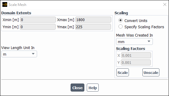
1. Select mm from the Mesh Was Created In drop-down list in the Scaling group box.
2. Click Scale.
3. Ensure that m is selected from the View Length Unit In drop-down list.
4. Ensure that Xmax and Ymax are reset to 1.8 m and 0.225 m respectively.
  The default SI units will be used in this tutorial, hence there is no need to change any units in this problem.
5. Close the Scale Mesh dialog box.
Check the mesh.
Domain → Mesh → Check → Perform Mesh Check
Note: You should check the mesh after you manipulate it (scale, convert to polyhedra, merge, separate, fuse, add zones, or smooth and swap). This will ensure that the quality of the mesh has not been compromised.
Display mesh with the default settings.
Domain → Mesh → Display...
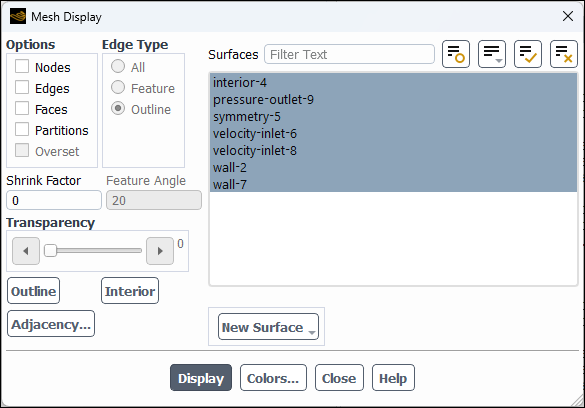
Examine the mesh.
Figure 16.2: The Quadrilateral Mesh for the Combustor Model

Note: You can use the right mouse button to probe for mesh information in the graphics window. If you click the right mouse button on any node in the mesh, information will be displayed in the Ansys Fluent console about the associated zone, including the name of the zone. This feature is especially useful when you have several zones of the same type and you want to distinguish between them quickly.
In the General task page, select Axisymmetric in the 2D Space list (Solver group box).
Setup → General

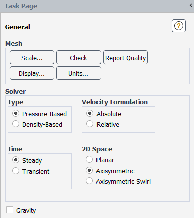
Ansys Fluent will display a warning about the symmetry zone in the console. You may have to scroll up to see this warning.
```
Warning: It appears that symmetry zone 5 should actually be an axis
                (it has faces with zero area projections).
                Unless you change the zone type from symmetry to axis,
                you may not be able to continue the solution without
                encountering floating point errors.
```
In the axisymmetric model, the boundary conditions should be such that the centerline is an axis type instead of a symmetry type. You will change the symmetry zone to an axis boundary in Boundary Conditions.

16.5.4. Models

Enable heat transfer by enabling the energy equation.
Physics → Models → Energy
Retain the default k-ω SST turbulence model.
Physics → Models → Viscous...
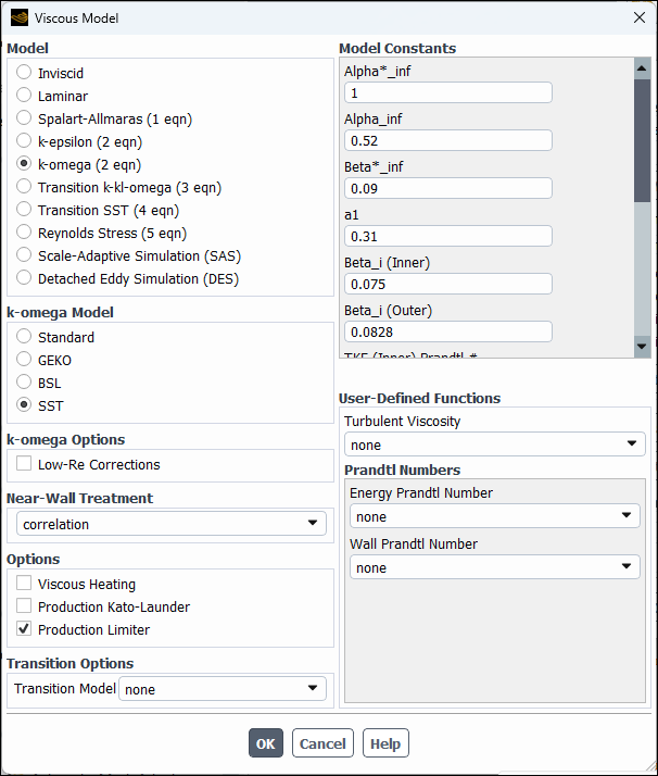
1. Retain the default settings for the k-omega model.
2. Click OK to close the Viscous Model dialog box.
Enable chemical species transport and reaction.
Physics → Models → Species...
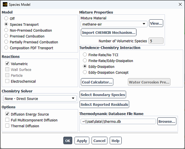
1. Select Species Transport in the Model list.
  The Species Model dialog box will expand to provide further options for the Species Transport model.
2. Enable Volumetric in the Reactions group box.
3. Select methane-air from the Mixture Material drop-down list.
  Scroll down the list to find methane-air.
  Note: The Mixture Material list contains the set of chemical mixtures that exist in the Ansys Fluent database. You can select one of the predefined mixtures to access a complete description of the reacting system. The chemical species in the system and their physical and thermodynamic properties are defined by your selection of the mixture material. You can alter the mixture material selection or modify the mixture material properties using the Create/Edit Materials dialog box (see Materials).
4. Select Eddy-Dissipation in the Turbulence-Chemistry Interaction group box.
  The eddy-dissipation model computes the rate of reaction under the assumption that chemical kinetics are fast compared to the rate at which reactants are mixed by turbulent fluctuations (eddies).
5. Click OK to close the Species Model dialog box.

16.5.5. Materials

In this step, you will examine the default settings for the mixture material. This tutorial uses mixture properties copied from the Fluent Database. In general, you can modify these or create your own mixture properties for your specific problem as necessary.

Confirm the properties for the mixture materials.
Setup → Materials → Mixture → methane-air Edit...
The Create/Edit Materials dialog box will display the mixture material (methane-air) that was selected in the Species Model dialog box. The properties for this mixture material have been copied from the Fluent Database... and will be modified in the following steps.
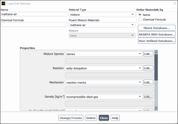
1. Click the Edit... button to the right of the Mixture Species drop-down list to open the Species dialog box.
  
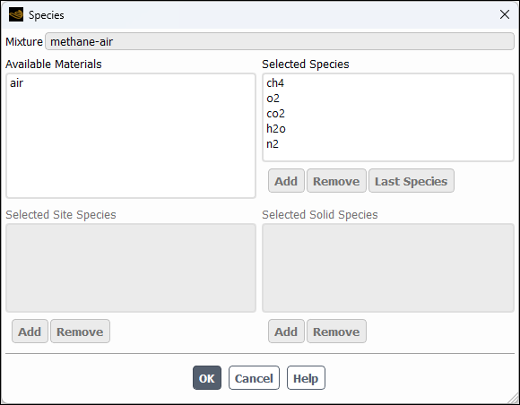
  You can add or remove species from the mixture material as necessary using the Species dialog box.
  1. Retain the default selections from the Selected Species selection list.
    The species that make up the methane-air mixture are predefined and require no modification.
  2. Click OK to close the Species dialog box.
2. Click the Edit... button to the right of the Reaction drop-down list to open the Reactions dialog box.
  
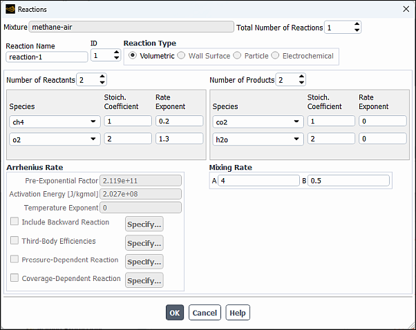
  The eddy-dissipation reaction model ignores chemical kinetics (the Arrhenius rate) and uses only the parameters in the Mixing Rate group box in the Reactions dialog box. The Arrhenius Rate group box will therefore be inactive. The values for Rate Exponent and Arrhenius Rate parameters are included in the database and are employed when the alternate finite-rate/eddy-dissipation model is used.
  1. Retain the default values in the Mixing Rate group box.
  2. Click OK to close the Reactions dialog box.
3. Retain the selection of incompressible-ideal-gas from the Density drop-down list.
4. Retain the selection of mixing-law from the Cp (Specific Heat) drop-down list.
5. Retain the default values for Thermal Conductivity, Viscosity, and Mass Diffusivity.
6. Click Change/Create to accept the material property settings.
7. Close the Create/Edit Materials dialog box.
The calculation will be performed assuming that all properties except density and specific heat are constant. The use of constant transport properties (viscosity, thermal conductivity, and mass diffusivity coefficients) is acceptable because the flow is fully turbulent. The molecular transport properties will play a minor role compared to turbulent transport.

16.5.6. Boundary Conditions

Convert the symmetry zone to the axis type.
Setup → Boundary Conditions → Symmetry → symmetry-5 Type axis
The symmetry zone must be converted to an axis to prevent numerical difficulties where the radius reduces to zero.
Set the boundary conditions for the air inlet (velocity-inlet-8).
Setup → Boundary Conditions → Inlet → velocity-inlet-8 Edit...
To determine the zone for the air inlet, display the mesh without the fluid zone to see the boundaries. Use the right mouse button to probe the air inlet. Ansys Fluent will report the zone name (velocity-inlet-8) in the console.
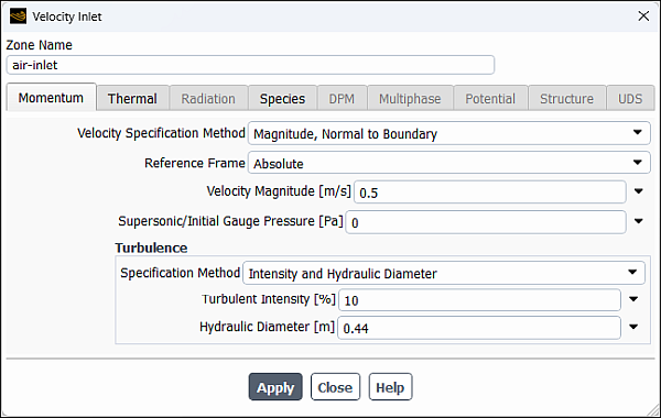
1. Enter air-inlet for Zone Name.
  This name is more descriptive for the zone than velocity-inlet-8.
2. Enter 0.5 for Velocity Magnitude.
3. Select Intensity and Hydraulic Diameter from the Specification Method drop-down list in the Turbulence group box.
4. Enter 10% for Turbulent Intensity.
5. Enter 0.44 for Hydraulic Diameter.
6. Click the Thermal tab and retain the default value of 300 for Temperature.
7. Click the Species tab and enter 0.23 for o2 in the Species Mass Fractions group box.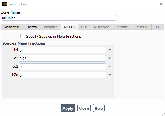
8. Click Apply and close the Velocity Inlet dialog box.
Set the boundary conditions for the fuel inlet (velocity-inlet-6).
Setup → Boundary Conditions → Inlet → velocity-inlet-6 Edit...
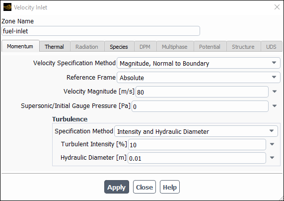
1. Enter fuel-inlet for Zone Name.
  This name is more descriptive for the zone than velocity-inlet-6.
2. Enter 80 for the Velocity Magnitude.
3. Select Intensity and Hydraulic Diameter from the Specification Method drop-down list in the Turbulence group box.
4. Enter 10% for Turbulent Intensity.
5. Enter 0.01 for Hydraulic Diameter.
6. Click the Thermal tab and retain the default value of 300 for Temperature.
7. Click the Species tab and enter 1 for ch4 in the Species Mass Fractions group box.
8. Click Apply and close the Velocity Inlet dialog box.
Set the boundary conditions for the exit boundary (pressure-outlet-9).
Setup → Boundary Conditions → Outlet → pressure-outlet-9 Edit...
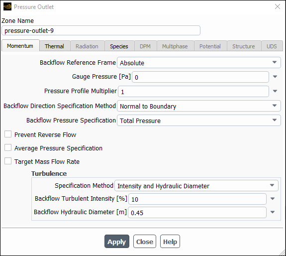
1. Retain the default value of 0 for Gauge Pressure.
2. Select Intensity and Hydraulic Diameter from the Specification Method drop-down list in the Turbulence group box.
3. Enter 10% for Backflow Turbulent Intensity.
4. Enter 0.45 for Backflow Hydraulic Diameter.
5. Click the Thermal tab and retain the default value of 300 for Backflow Total Temperature.
6. Click the Species tab and enter 0.23 for o2 in the Backflow Species Mass Fractions group box.
7. Click Apply and close the Pressure Outlet dialog box.
The Backflow values in the Pressure Outlet dialog box are utilized only when backflow occurs at the pressure outlet. Always assign reasonable values because backflow may occur during intermediate iterations and could affect the solution stability.
Set the boundary conditions for the outer wall (wall-7).
Setup → Boundary Conditions → Wall → wall-7 Edit...
Use the mouse-probe method described for the air inlet to determine the zone corresponding to the outer wall.
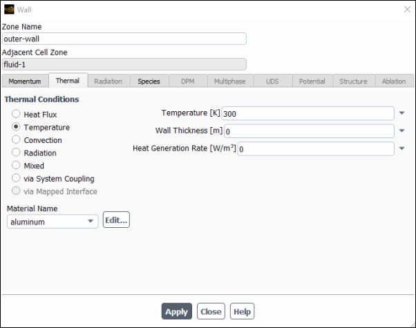
1. Enter outer-wall for Zone Name.
  This name is more descriptive for the zone than wall-7.
2. Click the Thermal tab.
  1. Select Temperature in the Thermal Conditions list.
  2. Retain the default value of 300 for Temperature.
3. Click Apply and close the Wall dialog box.
Set the boundary conditions for the fuel inlet nozzle (wall-2).
Setup → Boundary Conditions → Wall → wall-2 Edit...
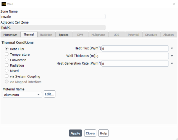
1. Enter nozzle for Zone Name.
  This name is more descriptive for the zone than wall-2.
2. Click the Thermal tab.
  1. Retain the default selection of Heat Flux in the Thermal Conditions list.
  2. Retain the default value of 0 for Heat Flux, so that the wall is adiabatic.
3. Click Apply and close the Wall dialog box.

16.5.7. Initial Reaction Solution

You will first calculate a solution for the basic reacting flow neglecting pollutant formation. In a later step, you will perform an additional analysis to simulate NOx.

Solution → Solution → Methods...

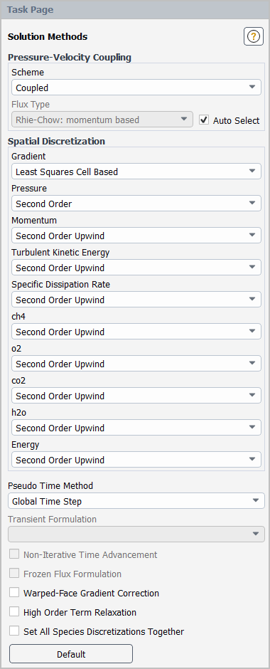
Retain the default selections.
Ensure the plotting of residuals during the calculation.
Solution → Reports → Residuals...
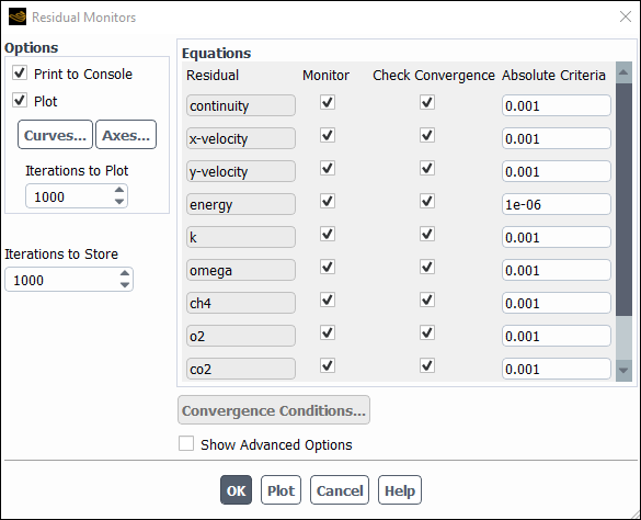
1. Ensure that Plot is enabled in the Options group box.
2. Click OK to close the Residual Monitors dialog box.
Initialize the field variables.
Solution → Initialization
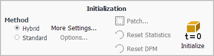
1. Retain the default Hybrid initialization method and click Initialize to initialize the variables.
Save the case file (gascomb1.cas.h5).
File → Write → Case...
1. Enter gascomb1.cas.h5 for Case File.
2. Click OK to close the Select File dialog box.
Run the calculation by requesting 200 iterations.
Solution → Run Calculation → Run Calculation...
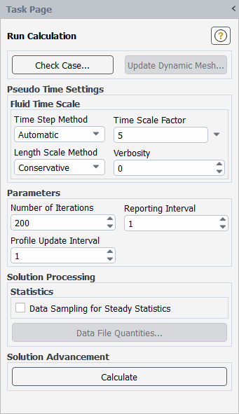
1. Enter 5 for the Time Scale Factor.
  The Time Scale Factor allows you to further manipulate the computed time step size calculated by Ansys Fluent. Larger time steps can lead to faster convergence. However, if the time step is too large it can lead to solution instability.
2. Enter 200 for Number of Iterations.
3. Click Calculate.
Save the case and data files (gascomb1.cas.h5 and gascomb1.dat.h5).
File → Write → Case & Data...
Note: If you choose a file name that already exists in the current folder, Ansys Fluent will ask you to confirm that the previous file is to be overwritten.

16.5.8. Postprocessing

Review the solution by examining graphical displays of the results and performing surface integrations at the combustor exit.

Report the total sensible heat flux.
Results → Reports → Fluxes...
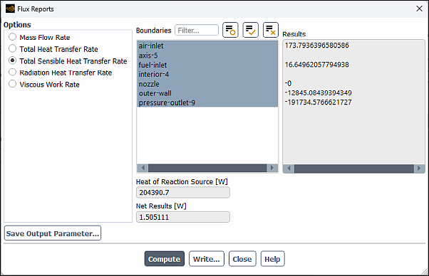
1. Select Total Sensible Heat Transfer Rate in the Options list.
2. Select all the boundaries from the Boundaries selection list (you can click the select-all button ).
3. Click Compute and close the Flux Reports dialog box.
  Note: The energy balance is good because the net result is small compared to the heat of reaction.
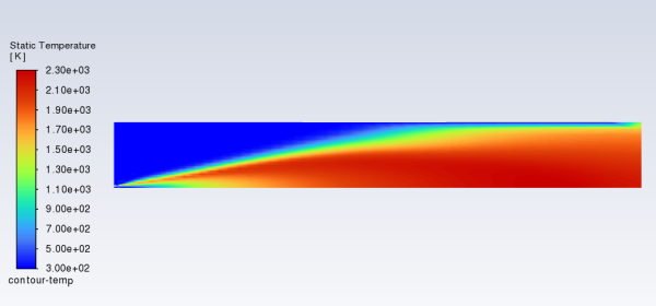
Display filled contours of temperature (Figure 16.3: Contours of Temperature).
Results → Graphics → Contours → New...
1. Enter contour-temp for Contour Name.
2. Ensure that Filled is enabled in the Options group box.
3. Select Banded in the Coloring group box.
4. Select Temperature... and Static Temperature in the Contours of drop-down lists.
5. Click Save/Display and close the Contours dialog box.
Figure 16.3: Contours of Temperature

The peak temperature is approximately 2300 .
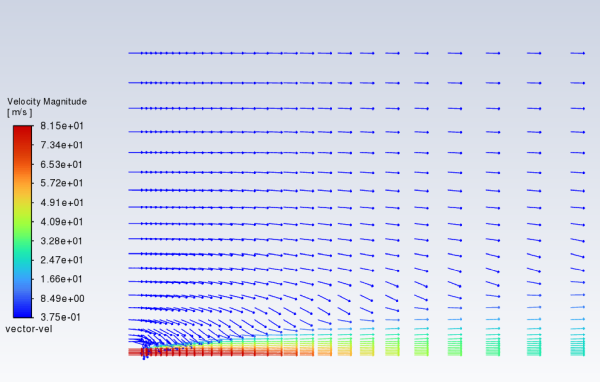
Display velocity vectors (Figure 16.4: Velocity Vectors).
Results → Graphics → Vectors → New...
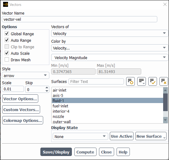
1. Enter vector-vel for Vector Name.
2. Select arrow from the Style drop-down list.
3. Enter 0.01 for Scale.
4. Click the Vector Options... button to open the Vector Options dialog box.
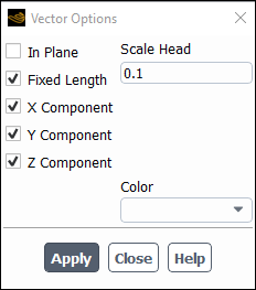
  1. Enable Fixed Length.
    The fixed length option is useful when the vector magnitude varies dramatically. With fixed length vectors, the velocity magnitude is described only by color instead of by both vector length and color.
  2. Enter 0.1 for Scale Head.
  3. Click Apply and close the Vector Options dialog box.
5. Click Save/Display and close the Vectors dialog box.
  The entrainment of air into the high-velocity methane jet is clearly visible.
Figure 16.4: Velocity Vectors
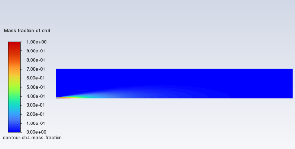
Display filled contours of mass fraction for (Figure 16.5: Contours of CH4 Mass Fraction).
Results → Graphics → Contours → New...
1. Enter contour-ch4-mass-fraction for Contour Name.
2. Select Species... and Mass fraction of ch4 from the Contours of drop-down lists.
3. Click Save/Display and close the Contours dialog box.
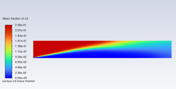
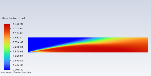
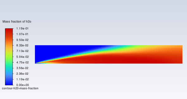
Figure 16.5: Contours of CH4 Mass Fraction
In a similar manner, display the contours of mass fraction for the remaining species , , and (Figure 16.6: Contours of O2 Mass Fraction, Figure 16.7: Contours of CO2 Mass Fraction, and Figure 16.8: Contours of H2O Mass Fraction).
Figure 16.6: Contours of O2 Mass Fraction

Figure 16.7: Contours of CO2 Mass Fraction

Figure 16.8: Contours of H2O Mass Fraction
Determine the average exit temperature.
Results → Reports → Surface Integrals...
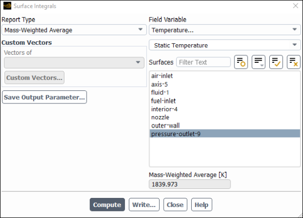
1. Select Mass-Weighted Average from the Report Type drop-down list.
2. Select Temperature... and Static Temperature from the Field Variable drop-down lists.
  The mass-averaged temperature will be computed as:
  (16–2)
3. Select pressure-outlet-9 from the Surfaces selection list, so that the integration is performed over this surface.
4. Click Compute.
  The Mass-Weighted Average field will show that the exit temperature is approximately 1840 .
Determine the average exit velocity.
Results → Reports → Surface Integrals...
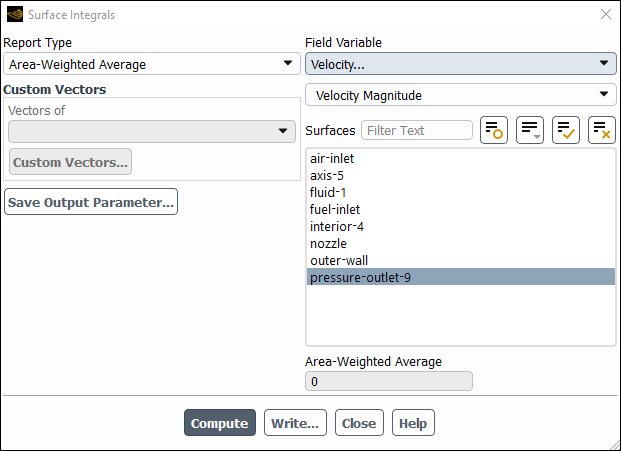
1. Select Area-Weighted Average from the Report Type drop-down list.
2. Select Velocity... and Velocity Magnitude from the Field Variable drop-down lists.
  The area-weighted velocity-magnitude average will be computed as:
  (16–3)
3. Click Compute.
  The Area-Weighted Average field will show that the exit velocity is approximately 3.37 .
4. Close the Surface Integrals dialog box.
Save the case file (gascomb1.cas.h5).
File → Write → Case...

16.5.9. NOx Prediction

In this section you will extend the Ansys Fluent model to include the prediction of NOx. You will first calculate the formation of both thermal and prompt NOx, then calculate each separately to determine the contribution of each mechanism.

Enable the NOx model.
Setup → Models → Species → NOx Edit...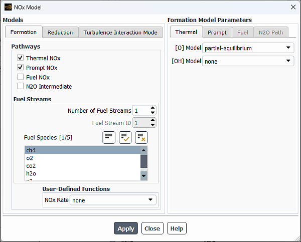
1. In the NOx Model dialog box, enable Thermal NOx and Prompt NOx in the Pathways group box.
  The dialog box expands to display the NOx model settings.
2. From the Fuel Species selection list, select ch4 (Fuel Streams group box).
3. Click the Turbulence Interaction Mode tab.
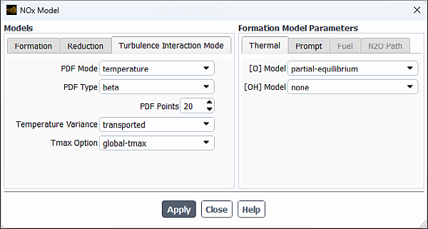
  1. Select temperature from the PDF Mode drop-down list.
    This enables the turbulence-chemistry interaction. If turbulence interaction is not enabled, you will be computing NOx formation without considering the important influence of turbulent fluctuations on the time-averaged reaction rates.
  2. Retain the default selection of beta from the PDF Type drop-down list and enter 20 for PDF Points.
    The value for PDF Points is increased from 10 to 20 to obtain a more accurate NOx prediction.
  3. Select transported from the Temperature Variance drop-down list.
4. Specify the formation model parameters (in the Formation Model Parameters group box).
  1. In the Thermal tab, select partial-equilibrium from the [O] Model drop-down list.
    The partial-equilibrium model is used to predict the O radical concentration required for thermal NOx prediction.
  2. In the Prompt tab, retain the default value of 1 for Fuel Carbon Number.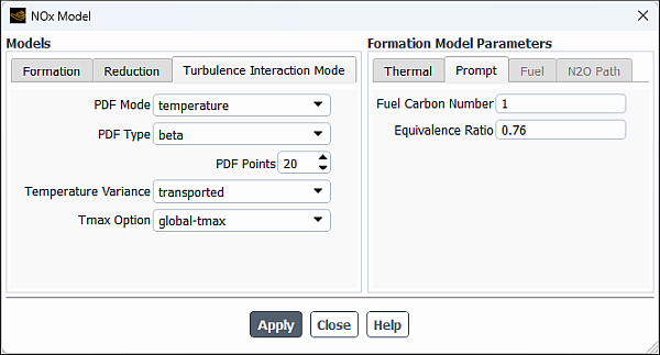
  3. Enter 0.76 for Equivalence Ratio.
    All of the parameters in the Prompt tab are used in the calculation of prompt NOx formation. The Fuel Carbon Number is the number of carbon atoms per molecule of fuel. The Equivalence Ratio defines the fuel-air ratio (relative to stoichiometric conditions).
5. Click Apply to accept these changes and close the NOx Model dialog box.
Enable the calculation of NO species and temperature variance only.
Solution → Controls → Equations...
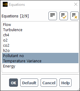
1. Deselect all variables except Pollutant no and Temperature Variance from the Equations selection list.
2. Click OK to close the Equations dialog box.
  You will predict NOx formation in a postprocessing mode, with the flow field, temperature, and hydrocarbon combustion species concentrations fixed. Hence, only the NO equation will be computed. Prediction of NO in this mode is justified on the grounds that the NO concentrations are very low and have negligible impact on the hydrocarbon combustion prediction.
Confirm the convergence criterion for the NO species equation.
Solution → Reports → Residuals...
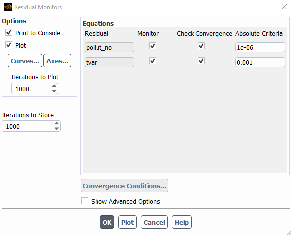
1. Ensure that the Absolute Criteria for pollut_no is set to 1e-06.
2. Click OK to close the Residual Monitors dialog box.
Request 25 more iterations.
Solution → Run Calculation
Save the new case and data files (gascomb2.cas.h5 and gascomb2.dat.h5).
File → Write → Case & Data...
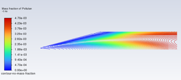
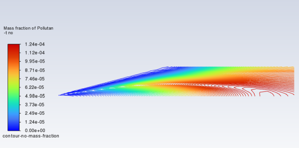
Review the solution by creating and displaying a contour definition for NO mass fraction (Figure 16.9: Contours of NO Mass Fraction — Prompt and Thermal NOx Formation).
Results → Graphics → Contours → New...
1. Enter contour-no-mass-fraction for Contour Name.
2. Disable Filled in the Options group box.
3. Select NOx... and Mass fraction of Pollutant no from the Contours of drop-down lists.
4. Click Save/Display and close the Contours dialog box.
  Figure 16.9: Contours of NO Mass Fraction — Prompt and Thermal NOx Formation
Calculate the average exit NO mass fraction.
Results → Reports → Surface Integrals...
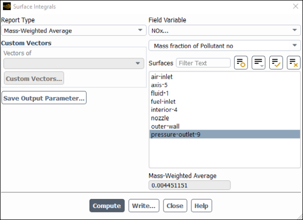
1. Select Mass-Weighted Average from the Report Type drop-down list.
2. Select NOx... and Mass fraction of Pollutant no from the Field Variable drop-down lists.
3. Ensure that pressure-outlet-9 is selected from the Surfaces selection list.
4. Click Compute.
  The Mass-Weighted Average field will show that the exit NO mass fraction is approximately 0.00445.
5. Close the Surface Integrals dialog box.
Save the case file (gascomb2.cas.h5).
File → Write → Case...
In the NOx Model dialog box, disable the prompt NOx mechanism in preparation for solving for thermal NOx only.
Setup → Models → Species → NOx Edit...
1. In the Formation tab, disable Prompt NOx.
2. Click Apply and close the NOx Model dialog box.
Request 25 iterations.
Solution → Run Calculation
Review the thermal NOx solution by displaying the contour-no-mass-fraction contour definition for NO mass fraction (under the Results/Graphics/Contours tree branch) you created earlier (Figure 16.10: Contours of NO Mass Fraction—Thermal NOx Formation).
Results → Graphics → Contours → contour-no-mass-fraction Display
Figure 16.10: Contours of NO Mass Fraction—Thermal NOx Formation

Note that the concentration of NO is slightly lower without the prompt NOx mechanism.
Compute the average exit NO mass fraction with only thermal NOx formation.
Results → Reports → Surface Integrals...

Tip: Follow the same procedure you used earlier for the calculation with both thermal and prompt NOx formation.

The Mass-Weighted Average field will show that the exit NO mass fraction with only thermal NOx formation (without prompt NOx formation) is approximately 0.00441.
Save the new case and data files (gascomb2-thermal.cas.h5 and gascomb2-thermal.dat.h5).
File → Write → Case & Data...
Solve for prompt NOx production only.
Setup → Models → Species → NOx Edit...
1. In the NOx Model dialog box, disable Thermal NOx (Pathways group box).
2. Enable Prompt NOx.
3. Click Apply and close the NOx Model dialog box.
Request 25 iterations.
Solution → Run Calculation
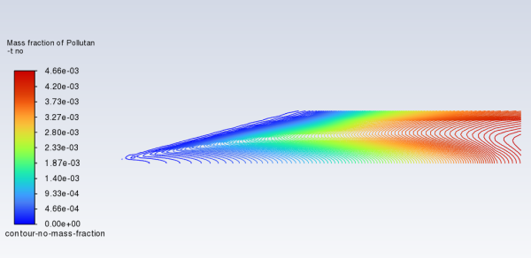
Review the prompt NOx solution by displaying the contour-no-mass-fraction contour definition for NO mass fraction (under the Results/Graphics/Contours tree branch) (Figure 16.11: Contours of NO Mass Fraction—Prompt NOx Formation).
Results → Graphics → Contours → contour-no-mass-fraction Display
Figure 16.11: Contours of NO Mass Fraction—Prompt NOx Formation

The prompt NOx mechanism is most significant in fuel-rich flames. In this case the flame is lean and prompt NO production is low.
Compute the average exit NO mass fraction only with prompt NOx formation.
Results → Reports → Surface Integrals...

Tip: Follow the same procedure you used earlier for the calculation with both thermal and prompt NOx formation.

The Mass-Weighted Average field will show that the exit NO mass fraction with only prompt NOx formation is approximately 9.87e-05
Note: The individual thermal and prompt NO mass fractions do not add up to the levels predicted with the two models combined. This is because reversible reactions are involved. NO produced in one reaction can be destroyed in another reaction.
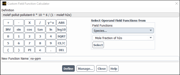
Use a custom field function to compute NO parts per million (ppm).
The NO ppm will be computed from the following equation:
(16–4)
Note: This is the dry ppm. Therefore, the value is normalized by removing the water mole fraction in the denominator.
User Defined → Field Functions → Custom...

Figure 16.12: The Custom Field Function Calculator Dialog Box
1. In the Custom Field Function Calculator dialog box, select NOx... and Mole fraction of Pollutant no from the Field Functions drop-down lists, and click the Select button to enter molef-pollut-pollutant-0 in the Definition field.
2. Click the appropriate calculator buttons to enter the following string in the Definition field (as shown in Figure 16.12: The Custom Field Function Calculator Dialog Box):
```
*10ˆ6/(1-
```
  Tip: If you make a mistake, click the DEL button on the calculator pad to delete the last item you added to the function definition.
3. From the Field Functions drop-down lists, select Species... and Mole fraction of h2o and click the Select button to enter molef-h2o in the Definition field.
4. Click the ) button to complete the field function.
5. Enter no-ppm for New Function Name.
6. Click Define to add the new field function to the variable list and close the Custom Field Function Calculator dialog box.
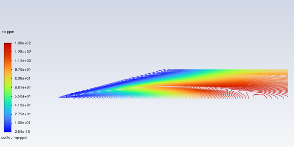
Display contours of NO ppm (Figure 16.13: Contours of NO ppm — Prompt NOx Formation).
Results → Graphics → Contours → New...
1. Enter contour-no-ppm for Contour Name.
2. Disable Filled in the Options group box.
3. Select Custom Field Functions... and no-ppm from the Contours of drop-down lists.
  Scroll up the list to find Custom Field Functions....
4. Click Save/Display and close the Contours dialog box.
Figure 16.13: Contours of NO ppm — Prompt NOx Formation

The contours closely resemble the mass fraction contours (Figure 16.11: Contours of NO Mass Fraction—Prompt NOx Formation), as expected.
Save the new case and data files (gascomb2-prompt.cas.h5 and gascomb2-prompt.dat.h5).
File → Write → Case & Data...

16.6. Summary

In this tutorial you used Ansys Fluent to model the transport, mixing, and reaction of chemical species. The reaction system was defined by using a mixture-material entry in the Ansys Fluent database. The procedures used here for simulation of hydrocarbon combustion can be applied to other reacting flow systems.

The NOx production in this case was dominated by the thermal NO mechanism. This mechanism is very sensitive to temperature. Every effort should be made to ensure that the temperature solution is not overpredicted, since this will lead to unrealistically high predicted levels of NO.

16.7. Further Improvements

Further improvements can be expected by including the effects of intermediate species and radiation, both of which will result in lower predicted combustion temperatures.

The single-step reaction process used in this tutorial cannot account for the moderating effects of intermediate reaction products, such as CO and . Multiple-step reactions can be used to address these species. If a multi-step Magnussen model is used, considerably more computational effort is required to solve for the additional species. Where applicable, the non-premixed combustion model can be used to account for intermediate species at a reduced computational cost.

For more details on the non-premixed combustion model, see the Fluent User's Guide.

Radiation heat transfer tends to make the temperature distribution more uniform, thereby lowering the peak temperature. In addition, radiation heat transfer to the wall can be very significant (especially here, with the wall temperature set at 300 ). The large influence of radiation can be anticipated by computing the Boltzmann number for the flow:

where is the Boltzmann constant (5.729 ) and is the adiabatic flame temperature. For a quick estimate, assume , , and (the majority of the inflow is air). Assume . The resulting Boltzmann number is Bo = 1.09, which shows that radiation is of approximately equal importance to convection for this problem.