Due to weight, structural and heating power limitations, Ice Protection Systems (IPS) only protect limited portions of aircraft surfaces. You may be inclined to model only the part of the structure associated with the IPS, however this approach may be problematic if the IPS allows running-wet conditions or is operating at off-design conditions. It is therefore a good practice to always consider a solid domain that includes portions of the structure extending downstream of the IPS enclosure, so that the inevitable runback effects and possible re-freeze of the liquid water film in the unprotected region can be adequately captured.

From the geometrical point of view, it is also very important to ensure that pairs of surfaces that form an interface are in contact with each other, are matching in size and shape and that the grid resolutions on either side of the interface are comparable. For example, the jets emanating from piccolo tube orifices form hot spots on the protected surface, and the associated flow phenomena exhibit very strong velocity and temperature gradients that should be captured with sufficient spatial resolution. In addition, the solid and external airflow grids also need to be refined in the region of the jet impingement location to prevent artificial diffusion of the heat fluxes and temperature gradients that would occur due to sudden grid density changes from one domain to the next. The CHT3D interface communication software is designed to support domains that may not be precisely in contact with one another or provide a perfect overlap. This is a common situation that arises when external and internal grids are generated by different teams in an organization. As long as the gap/overlap/penetration is smaller than the edges of the element faces, the data mapping algorithms can handle such non-conformities.

CHT simulations of typical aircraft IPS involve cold high-speed flows at high Reynolds numbers on the outer skin surfaces and sonic or supersonic regions in the hot-air inner chamber, therefore the flow and thermal gradients on either side of the interface are very large and require low-Reynolds number turbu- lence models that support laminar-to-turbulent flow transition, such as the SST intermittency model in FENSAP, Fluent or CFX, and the associated very fine grids for accuracy. To ensure sufficient accuracy, the thickness of the grid elements of the airflow domains in contact with the CHT interfaces expand gradually with the normal distance from the interface. Moreover, ensure the first layer of cells, above the interface and walls, have y⁺ values less than 1.

In piccolo tube applications, the hot-air jets impinge on relatively thin aluminum or titanium skins. It might be tempting to construct a solid skin domain composed of a single layer of elements, however in these applications the temperature gradients can be very large and some heat diffusion may occur in the metal skin, therefore a multi-layer grid is preferable. Furthermore, due to the small thickness of the metal skin, it may be more efficient to use structured grids that permit elongated elements.

C3D, the finite element heat conduction solver, is relatively insensitive to element aspect ratio. For solid grids, 3 to 5 element layers crossing the thin solid skin are recommended and should be sufficient for most applications.

Electro-thermal anti- and de-icing ice protection systems are typically built with multi-layer, multi-material composite skin assemblies, divided into multiple heating strips. The simulation of these arrangements usually involves a single (external) fluid domain. The same issues raised for piccolo tube applications, such as ensuring that the solid domain extends well past the protected region and that the surface mesh coverage is of very similar density on both sides of the interface also apply to these simulations.

The internal heated cavity airflow solution may be rather complex and may contain regions of high turbulence, high velocity and temperature gradients, such as the hot jets and the saucer-shaped rollup vortices that they produce, and will feature several strong recirculation zones. Suitably fine grids are therefore needed to ensure that these features are correctly captured.

OptiGrid (See OptiGrid - Mesh Adaptation) is the perfect tool to ensure that the grid can capture all these features accurately. The external airflow grid and the solid grid should have the same surface grid density, hence ideally when mesh adaptation is used the external and solid grids should be constructed after adapting the mesh of the heated cavity.

Before attempting wet-air CHT simulations (anti-icing or de-icing) with your setup, you should make sure the accuracy of dry-air results is within the acceptable range. This is to verify that the solid material properties, flow boundary conditions, heater power levels, location of temperature probes, and many other physical parameters that play a role in the simulation are correctly set, and the solvers are producing expected results. Mesh refinement, adaptation and turbulence model adjustments (for example, laminar-to-turbulent transition) may be necessary to fine tune the results. Once you are confident with the dry-air CHT process, you can move onto wet-air simulations.

Initial solutions are required for the internal and external fluid domains, droplets and surface liquid water film. These solutions can be obtained with isothermal or adiabatic wall conditions. The isothermal wall approach is the classical method where walls are set to +10 K of the expected stagnation temperature to generate measurable heat fluxes that will be converted to heat transfer coefficients by ICE3D. Starting with FENSAP-ICE version 2022 R2, it is possible to use adiabatic walls as well, which is to be accompanied by EID calculation in ICE3D step to extract the heat transfer coefficients. When using EID for external flow, vapor transport should also be enabled in DROP3D to provide accurate water vapor pressure distribution on the external surface. The adiabatic wall approach should be used if there are hot air exhausts entering the external flow domain and interacting with the icing surfaces.

Additionally, to accelerate the convergence of CHT3D, an initial ICE3D solution should be computed on the external domain to establish an initial water film coverage. Only the extent of the water film coverage on the external surface is sought, and can usually be established with a simulation of 20-30 seconds, depending on film speed and the streamwise length of the surface. In steady-state anti-icing CHT3D computations, any ice shapes produced by ICE3D are not representative of a real ice shape, since the ice mass and height are reset at the beginning of each CHT iteration. In these cases, ICE3D only computes the thermodynamic conditions governing the behavior the water on the skin surface. If a realistic ice shape for a specific duration is required, a single-shot ICE3D simulation or a multishot sequence simulation (MULTI-FENSAP and MULTI-FLUENT only) can be executed after the anti-icing CHT3D computation has converged.

De-icing simulations are performed as unsteady, using physical time steps that are usually in the order of 0.01 – 1 seconds. The non-linear interface problem is resolved with the help of sub-iterations within each time step. By default, these iterations are set to 10, which is a conservative value to ensure convergence. You could reduce this value to 3 to accelerate calculations if the minimum and maximum solid temperatures appear to have converged by then within each time step. This can be observed in the convergence graphs of CHT3D.

---

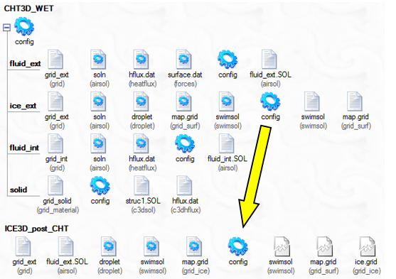
Note:  In the case of a single ICE3D simulation, a drag-&-drop of the config icon of the ice_ext component of the CHT3D run onto the config icon of the ICE3D run will automatically set the in-flight icing solution and the steady-state conductive (anti-icing) heat flux solution of the CHT3D run as inputs to the ICE3D run. This is supported when FENSAP, Fluent or CFX are used as airflow solvers.

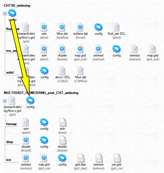
In the case of a multishot sequence simulation based on a CHT result, a drag-&-drop of the config icon of the CHT3D run onto the config icon of the multishot run will automatically take all reference conditions and thermal equilibrium solutions from each module of the CHT3D run and set them as inputs to their respective modules of the multishot run.

In both cases, the conductive (anti-icing) heat flux obtained during the CHT3D calculation is kept constant during the ice accretion process. A separate set of tutorials inside the FENSAP-ICE Tutorial Guide portrays these setups. This feature is currently supported in MULTI-FENSAP and MULTI-FLUENT but not in MULTI-CFX.

---

Conversely, if an unsteady de-icing simulation is conducted, the transient and final ice shape will be determined directly in the CHT3D computation.

Since the setup of a CHT simulation requires careful consideration and planning, it is advisable to consult the Ansys FENSAP-ICE Tutorial Guide for examples of how to create the various domain grids, the coverage of each interface, the boundary conditions, etc.