


Hexahedral Elements
The preferred element for solid bodies in Explicit Dynamics systems is the eight node reduced integration hexahedral. These elements are well suited to transient dynamic applications including large deformations, large strains, large rotations and complex contact conditions. The basic element characteristics are
| Connectivity | 8 Node |
 | |
| Nodal Quantities | Position, Velocity, Acceleration, Force |
| Mass (lumped mass matrix) | |
| Element Quantities | Volume, Density, Strain, Stress, Energy |
| Other material state variables | |
| Material Support | All available materials |
| Points to Note | Preferred element for Explicit Dynamics |
| Reduced integration, constant strain element | |
| Requires hourglass damping to stabilize zero energy "hourglass" modes (see section Damping Controls, Hourglass Damping) |
The default Integration Type for hexahedral elements is the Exact option. Here the element formulation based upon the work of Wilkins [8] results in an exact volume calculation even for distorted elements. This formulation is therefore the most accurate option, especially if the faces of the hex elements become warped. This is also computationally the most expensive formulation.
It is possible to speed-up simulations by using the 1pt Gaussian quadrature integrated hexahedral element. This uses the element formulation described by Hallquist [9]. There will be some loss in accuracy when using this formulation with warped element faces which are common place in large deformation analysis.
Tetrahedral Elements
Linear 4 noded tetrahedron elements are available for use in Explicit Dynamic analysis.
| Connectivity | 4 Node |
 | |
| Nodal Quantities | Position, Velocity, Acceleration, Force |
| Mass (lumped mass matrix) | |
| Additionally ANP formulation: Volume, Pressure, Energy | |
| Additionally NBS: Volume, Density, Strain, Stress, Energy, Pressure and other material state variables | |
| Element Quantities | Volume, Density, Strain, Stress, Energy |
| Other material state variables | |
| Additionally NBS: If PUSO stability coefficient is set to a non-zero value, there is an additional variable set for all variables for the PUSO solver | |
| Material Support | SCP: All available materials |
| Only Isotropic materials can be used with the ANP formulation | |
| Only ductile materials can be used with the NBS formulation | |
| Points to Note | Only the ANP and NBS are recommended for use in majority tetrahedral meshes |
| For NBS models exhibiting zero energy modes, the Puso coefficient can be set to a non-zero value. A value of 0.1 is recommended. | |
| Reduced integration, constant strain element |
The four noded linear tetrahedron is available with three forms of Pressure Integration
The SCP tetrahedral element is a basic, constant strain element and can be used with all the material models. The element is intended as a "filler" element in meshes dominated by hexahedral elements. The element is known to exhibit locking behavior under both bending and constant volumetric straining (that is, plastic flow). If possible the element should therefore not be used in such cases.
The ANP tetrahedral formulation used here is an extension of the advanced tetrahedral element (Burton [11]) and can be used as a majority element in the mesh. The ANP tetrahedral overcomes problems of volumetric locking.
The NBS tetrahedral formulation based on the work of (Bonet [21] and Puso [22]) is a further extension of the ANP tetrahedral element and can also be used as a majority element in the mesh. The NBS tetrahedral overcomes both problems of volumetric and shear locking, therefore is recommended over the other two tetrahedral formulations for models involving bending.
Supported material types in the NBS tetrahedral element are currently limited to ductile materials. The following is a list of supported material properties for NBS tetrahedral elements:
Isotropic Elasticity
Bulk Modulus
Shear Modulus
Polynomial EOS
Shock EOS
Johnson Cook Strength
Zerilli Armstrong Strength
Cowper Symonds Strength
Steinberg Guinan Strength
Bilinear Isotropic Hardening
Multilinear Isotropic Hardening
Tensile Pressure Failure
Plastic Strain Failure
Principal Stress Failure
Principal Strain Failure
Principal Stress/Principal Strain Failure
Grady Spall Failure
Johnson Cook Failure
Stochastic Failure
Note: Both flexible and rigid bodies are supported for NBS tetrahedral elements.
If a model containing NBS tetrahedral elements exhibits zero-energy modes (Puso, 2006 [22]), the PUSO stability coefficient can be set to a non-zero value. The recommended value is 0.1. Stabilization is achieved by taking a contribution to the nodal stresses from the SCP solution. Therefore, for models with a non-zero Puso stability coefficient, the solution is computed on both the nodes and the elements.
NBS tetrahedral elements cannot share nodes with ANP tetrahedral elements, SCP tetrahedral elements, shell elements, or beam elements. Also note that the use of NBS tetrahedral elements with joins or spotwelds is not supported.
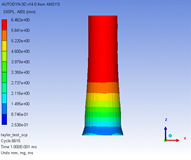
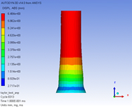
Figure 10.7: Comparison of results of a Taylor test solved using SCP, ANP and NBS Tetrahedral elements. Results using NBS and ANP tetrahedral elements compare more favorably with experimental results than results using SCP (see table below).
| Tet-SCP | Tet-ANP | Tet-NBS |
|---|---|---|
 |
 |
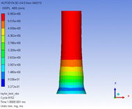 |
Table 10.3: Comparison of the performance of SCP, ANP, NBS and hex elements in a model involving bending. The displacement of the beam with NBS tetrahedral elements is the most similar to the beam meshed with hexahedral elements as it does not exhibit shear locking as is seen in the beams solved using SCP and ANP tetrahedral elements.
|
Experiment |
SCP Tet |
ANP Tet |
NBS Tet | |
|---|---|---|---|---|
|
Cylinder length (mm) |
31.84 |
30.98 |
30.97 |
31.29 |
|
Impact diameter (mm) |
12.0 |
10.66 |
11.32 |
11.28 |
Figure 10.8: Example bending test using SCP (1), ANP (2), NBS tetrahedral (3), and hex (4) elements. The displacement of the beam with NBS tetrahedral elements is the most similar to the beam meshed with hexahedral elements as it does not exhibit shear locking.
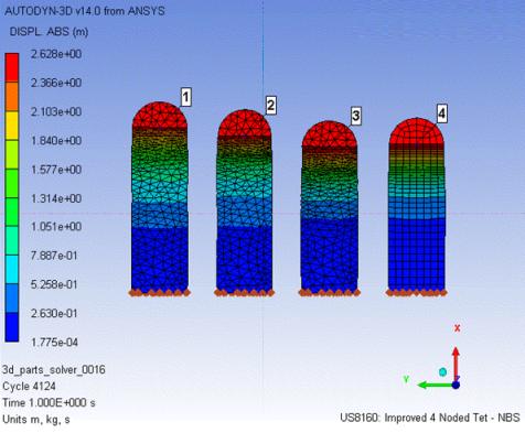
Figure 10.9: Taylor test: Iron cylinder impacting rigid wall at 221m/s. Good correlation between ANP and Hex element results is obtained
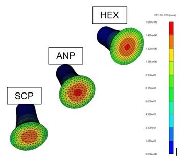

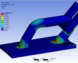
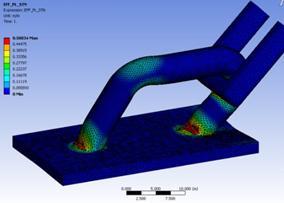
Figure 10.10: Example pull out test simulated using both hexahedral elements and ANP tetrahedral elements. Similar plastic strains and material fracture are predicted for both element formulations used.
 |
 |
Pentahedral Elements
Linear 6 noded pentahedral elements are available for use in Explicit Dynamics analysis.
| Connectivity | 6 Node |
 | |
| Nodal Quantities | Position, Velocity, Acceleration, Force |
| Mass (lumped mass matrix) | |
| Element Quantities | All available materials |
| Other material state variables | |
| Material Support | All available materials |
| Points to Note | Reduced integration, constant strain element |
The pentahedral element is a basic constant strain element and is intended as a filler element in meshes dominated by hexahedral elements.
Pyramid Elements
Pyramid elements are not recommended for Explicit Dynamics simulations. Any pyramid elements present in the mesh will be converted to 2 tetrahedral elements in the solver initialization phase. Results are mapped back onto the Pyramid element for postprocessing purposes.
Shell Quad Elements
Bilinear 4 noded quadrilateral shell elements are available for use in Explicit Dynamics analysis.
| Connectivity | 4 Node |
 | |
| Nodal Quantities | Position, Velocity, Angular Velocity, Acceleration, Force, Moment |
| Mass (lumped mass matrix) | |
| Element Quantities | Strain, Stress, Energy |
| Other material state variables | |
| Data stored per layer | |
| Material Support | Linear elasticity must be used |
| Equations of state and porosity are not applicable to shell elements | |
| Pressure dependant material strength is not applicable to shell elements | |
| Points to Note | Reduced integration, constant strain element |
| Based on Mindlin plate theory, transverse shear deformable | |
| Shells have zero through thickness stress and are therefore not suitable for modelling wave propagation through the thickness of the surface body |
The bilinear 4 noded quadrilateral shell element is based on the corotational formulation presented by Belytschko-Tsay [13]. The element has one quadrature point per layer and is stabilized using hourglass control. By default, additional curvature terms are added for warped elements in accordance with Belytschko [14]. This option is deactivated using the Shell BWC Warp Correction setting in the Solver Controls.
The number of through thickness integration points (sublayers) is controlled through the analysis settings option Solver Controls, Shell Sublayers. The default value is 3.
The thickness of the shell element is updated during the simulation in accordance with the material response. The update is carried out at the shell nodes by default.
The principal inertia of the shell nodes is recalculated every time increment (cycle) by default. This is the most robust method. It is more efficient to rotate the principal inertias rather than recalculate (although less robust for certain applications). The Shell Thickness Update option can be used to select this more efficient inertial update method.
Shell Tri Elements
Linear 3 noded triangular shell elements are available for use in Explicit Dynamics analysis.
| Connectivity | 3 Node |
 | |
| Nodal Quantities | Position, Velocity, Angular Velocity, Acceleration, Force, Moment |
| Mass (lumped mass matrix) | |
| Element Quantities | Volume, Density, Stress, Energy |
| Other material state variables | |
| Data stored per layer | |
| Material Support | Linear elasticity must be used |
| Equations of state and porosity are not applicable to shell elements | |
| Pressure dependant material strength is not applicable to shell elements | |
| Points to Note | Reduced integration, constant strain element |
| This element is only recommended for use as a "filler" element in quad dominant shell meshes | |
| Shells have zero through thickness stress and are therefore not suitable for modelling wave propagation through the thickness of the surface body |
The bilinear 3 noded, C0, triangular shell element is based on the formulation presented by Belytschko et al. [15]. The number of through thickness integration points (sublayers) is controlled through the analysis settings option Solver Controls, Shell Sublayers. The default value is 3.
The thickness of the shell element is updated during the simulation in accordance with the material response. The update is carried out at the element irrespective of the global settings for Shell Thickness update in Mechanical.
Beam Elements
Linear 2 noded beam elements are available for use in Explicit Dynamics analysis.
| Connectivity | 2 Node |
 | |
| Nodal Quantities | Position, Velocity, Angular Velocity, Acceleration, Force, Moment |
| Mass (lumped mass matrix) | |
| Element Quantities | Resultant Strain/Stress, Energy |
| Other material state variables | |
| Material Support | Linear elasticity must be used |
| Equations of state and porosity are not applicable to beam elements | |
| Pressure dependant material strength is not applicable to beam elements | |
| Points to Note | Supports symmetrical circular, square, rectangular, I-Beam and general cross sections |
| Beams have zero transverse stress and are therefore not suitable for modeling wave propagation across the cross section |
The 2 noded beam element is based on the resultant beam formulation of Belytschko [16] and allows for large displacements and resultant elasto-plastic response.
SPH Elements
Bodies meshed with the particle method are solved using the Smoothed Particle Hydrodynamics (SPH) method. SPH characteristics are summarized in the table below:
| Connectivity | Mesh Free |
| Particle Quantities |
Position, Velocity, Acceleration, Force Mass Resultant Stress/Strain, Energy Other material state variables |
| Material Support | All available, but thermal conductivity not supported |
| Points to Note |
Lagrangian formulation using cubic spline kernel function Suitable for applications which would result in large mesh distortion or tangling if using solid elements Take note of tensile instabilities. |
The default values for the SPH options in the analysis settings should be sufficient for most examples, but it may be necessary to change them to improve the accuracy of solutions for certain types of applications.