


Treatment of Shock Discontinuities
Strong impacts on solid bodies can give rise to the formation of shock waves in the material. Because of the nonlinearity of the equations being solved, shocks can form even though the initial conditions are smooth.
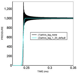
In order to handle the discontinuities in the flow variables associated with such shocks, viscous terms are introduced into the solutions. These additional terms have the effect of spreading out the shock discontinuities over several elements and thus allow the simulation to continue to compute a smooth solution, even after shock formation and growth.
Figure 10.5: Comparison of pressure solution at a shock wave discontinuity a) using no artificial viscosity b) using the default artificial viscosity
The viscous terms used in the Explicit Dynamics system is based on the work of von Neumann and Richtmyer [4] and Wilkins [5].
 | (10–20) |
Where
CQ is the Quadratic Artificial Viscosity coefficient
CL is the Linear Artificial Viscosity coefficient
ρ is the local material density
d is a typical element length scale
c is the local sound speed
 is the rate in change of volume
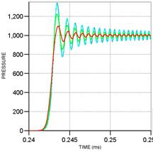
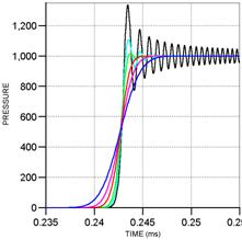
The quadratic term smooths out shock discontinuities while the linear term acts to damp out oscillations which may occur in the solution behind the shock discontinuity.
Figure 10.6: Effects of artificial viscosity on the solution
 |
 |
|
a) Quadratic term stabilizes |
b) The linear term reduces noise |
Note:
The pseudo-viscous term is usually added only when the flow is compressing. The Linear Viscosity in Expansion option can be used to apply the pseudo-viscous term in both compression and expansion. This can lead to excessive dispersion in the solution.
The inclusion of the pseudo-viscous pressure imposes further restrictions on the time step in order to ensure stability:
Due to the quadratic term,

Due to the linear term,

The resulting critical time step is

The pseudo-viscous pressure is stored for each element and can be contoured using the custom variable VISC_PRESSURE
For SPH bodies, the default formulation of artificial viscosity used is a Monaghan type artificial viscosity (as discussed in the work of Liu and Liu [23]), which takes the form:
 | (10–21) |
where  and
and  are the linear and quadratic constants (specific to SPH) and
 | (10–22) |
This is the recommended viscosity formulation to use, as it was formulated specifically for SPH. It is possible to use the Neumann and Richtmyer form of Artificial Viscosity for SPH using a beta command snippet. Details of the command snippet are found in Command Objects for SPH Settings.
Hourglass Damping
The reduced integration eight node hexahedral elements, or 4 node quadrilateral elements, used in Explicit Dynamics can exhibit "hourglass" modes of deformation.
Since the expressions for strain rates and forces involve only differences in velocities and/or coordinates of diagonally opposite nodes of the cuboidal element, if the element distorts in such a way that these differences remain unchanged there will be no strain increase in the element and therefore no resistance to this distortion. Hourglass modes of deformation occur with no change in energy (also called zero energy modes) and are unphysical.
An example of such a distortion in two dimensions is illustrated below where the two diagonals remain the same length even though the cell distorts.
Visualization in three dimensions is much more difficult but if such distortions occur in a region of many elements, patterns such as that shown below occur and the reason for the name of "hourglass instability" is more easily understood.
To avoid these zero energy modes of deformation from occurring, corrective forces (Hourglass forces) are added to the solution to resist the hourglass modes of deformation.
Hexahedral Elements
Two formulations for calculating the Hourglass forces are available for Hexahedral elements:
The Standard formulation is based on the work of Kosloff and Frazier [6] and generates hourglass forces proportional to nodal velocity differences. This is often referred to as a viscous formulation.
 | (10–23) |
Where
FH is a vector of the hourglass forces at each node of the element
CH is the Viscous Coefficient for hourglass damping
ρ is the material density
c is the material soundspeed
V is the material volume
 is a vector function of the element nodal velocities aligned with the
hourglass shape vector
is a vector function of the element nodal velocities aligned with the
hourglass shape vector
The standard formulation is the most efficient formulation in terms of CPU and is therefore the default option. It is not however invariant under rigid body rotation (i.e. under rigid body rotation the hourglass forces may not sum to zero)
The Flanagan Belytschko [7] formulation is invariant under rigid body rotation and is therefore recommended for simulations in which large rotations of hexahedral elements are expected. The Flanagan Belytschko formulation is similar to the standard form.
 | (10–24) |
The difference lies in the construction of the vector function of element nodal velocities,
 . These are constructed to be orthogonal to both linear velocity field and the
rigid body field.
. These are constructed to be orthogonal to both linear velocity field and the
rigid body field.
Note:
The Viscous Coefficient for hourglass forces usually varies between 0.05 and 0.15. The default value is 0.1.
The sum of the hourglass forces applied to an element is normally zero. The momentum of the system is therefore unaffected by hourglass forces.
The hourglass forces do however do work on the nodes of the elements. The energy associated with hourglass forces is a) stored locally in the specific internal energy of the element b) recorded globally over the entire model and available to review via the Solution Output, Energy Summary.
When using Flanaghan-Belytschko hourglass control, further restrictions are imposed on the stability time step based on the maximum eigenfrequency of the element. See Flanagan Belytschko [7] for further information.
Static Damping
The Explicit Dynamics system is primarily designed for solving transient dynamic events. Using the static damping option, a static equilibrium solution can also be obtained.
The procedure is to introduce a damping force which is proportional to the nodal velocities and which is aimed to critically damp the lowest mode of oscillation of the static system. The solution is then computed in time in the normal manner until it converges to an equilibrium state. The user is required to judge when the equilibrium state is achieved. If the lowest mode of the system has period T then we may expect the solution to converge to the static equilibrium state in a time roughly 3T if the value of T is that for critical damping.
When the dynamic relaxation option is used the velocity update is modified to
 | (10–25) |
where the Static Damping Coefficient, Rd , is input by the user. The value of Rd for critical damping of the lowest mode is
 | (10–26) |
where T is the period of the lowest mode of vibration of the system (or a close approximation to it). Usually
 | (10–27) |
A reasonable estimate of T must be used to ensure convergence to an equilibrium state but if the value of T is not known accurately then is it recommended that the user overestimates it, rather than underestimating it. Approximate values of Δt and T can usually be obtained by first performing a dynamic analysis without static damping.
A static damping coefficient may be defined, or removed, at any point during an Explicit Dynamic simulation. Typical examples of its use would be:
To establish an initial stress distribution in a structure, prior to solving a transient dynamic event. For example applying gravity to a structure.
To establish the final static equilibrium position of a structure after it has experienced a transient dynamic event. For example finding the equilibrium position of structure after it has undergone large plastic deformation during a dynamic event.