


Important: Note that beta features have not been fully tested and validated. Ansys, Inc. makes no commitment to resolve defects reported against these prototype features. However, your feedback will help us improve the overall quality of the product. We will not guarantee that the projects using this beta feature will run successfully when the feature is finally released so you may, therefore, need to modify the projects.
The behavior of liquids, such as water, is often modeled as single-phase and free-surface flows. However, the presence of surrounding air can significantly influence the behavior of liquids.
The SPH Air Drag (Beta) module estimates and applies the drag force caused by surrounding air flowing at constant velocity onto a liquid flow simulated with SPH.
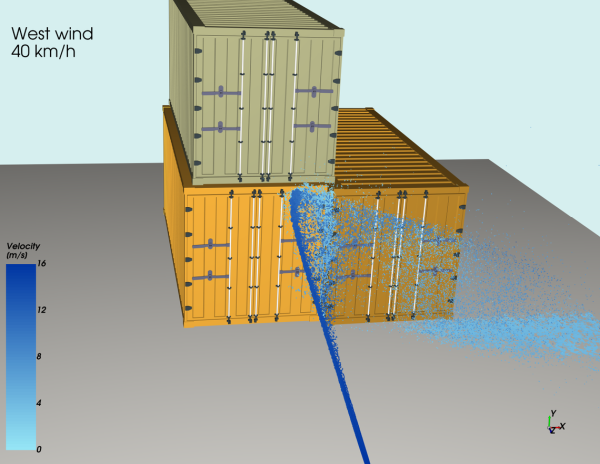
An application of the SPH Air Drag (Beta) module is demonstrated in Figure 40.1: Example application of the SPH Air Drag (Beta) module in a fire hose jet scenario., where a simulation of a jet of water from a fire hose is performed using the SPH solver. In this scenario, the module is utilized to incorporate the influence of a constant westward wind at a velocity of 40 km/hr.
By employing this one-way coupled model, it becomes possible to evaluate the impact of varying wind velocities and directions on the cooling pattern of the surrounding container.
The SPH Air Drag (Beta) module follows a simplified approach to model the effects of air, without the need of representing it with another SPH phase. The SPH Air Drag (Beta) module models the drag forces exerted by an air phase, with constant and predefined velocities, onto the free surface of the SPH fluid based on the work of [38]. The model accounts for the exposed surface area of each SPH element and approximates its deformation to improve the drag force estimation.
While the SPH Air Drag (Beta) module effectively models the effects of air without representing it as SPH elements, there are several limitations that should be taken into consideration.
Uniform air velocity throughout the domain: the air velocity is constant and uniform throughout the domain and its effects may be sensed by all SPH elements in the entire domain.
Inability to reproduce entrapped air effects: the module cannot accurately reproduce effects associated with entrapped air, such as rising air bubbles. These phenomena are not accounted for in the simulation due to the absence of a fully simulated air phase.
One-Way coupling and limited fluid-to-air interactions: since the module operates with a one-way coupling approach, interactions where the fluid influences the air cannot be accurately modeled. The module focuses primarily on the effect of air on the fluid, without considering the reciprocal influence.
Lack of turbulent behavior and lift effects: as the module does not simulate the air phase, it cannot capture turbulent behavior or lift effects. These features, which are essential for simulating scenarios like a flying airplane, are not accounted for in the current implementation.
This module has several parameters that you can set, as shown in Figure 40.2: SPH Air Drag (Beta) module options..
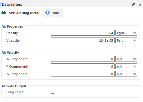
These parameters are explained below:
Air Properties: The required list of properties of the air phase.
Density: This defines the density of the air phase.
Range: [Positive values]
Viscosity: This defines the dynamic viscosity of the air phase.
Range: [Positive values]
Air Velocity: The constant velocity vector of the air field, the magnitude of which is made up of the x, y, and z components respectively.
X-Component: Air velocity component in the x-direction.
Range: [Any Value]
Y-Component: Air velocity component in the y-direction.
Range: [Any Value]
Z-Component: Air velocity component in the z-direction.
Range: [Any Value]
Activate Output: This defines the outputs of the module. Depending on the selection of the items below, additional properties are created for each SPH element and can be used for post-processing.
Drag Force: When enabled, the drag force exerted by the air will be added as an additional property of the SPH elements. When cleared, the drag force due to the air phase will not be available for post-processing.
Range: [Turns on or off]
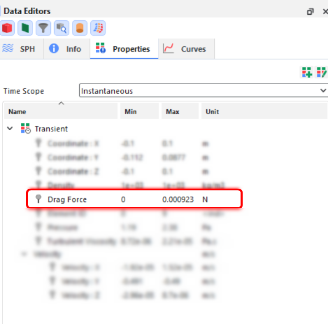
If the Drag Force was selected in the Activate Output in the Data Editor of the SPH Air Drag (Beta) module, a new property will be available for the main SPH entity, as shown in Figure 40.3: Additional property enabled on the SPH entity when the SPH Air Drag (Beta) is used..
You can choose to analyze this property in a plot or histogram window., or display this property graphically in a 3D View window.
This additional property is explained below:
Drag Force: This provides the drag force acting on each SPH element due to the interaction with the surrounding air phase, which can help you to visualize how the liquid phase is affected by the air phase.
Ensure that the module is enabled. Go to the Data panel, select Modules, and make sure the SPH Air Drag (Beta) checkbox is enabled in the Data Editors panel.
Select SPH Air Drag (Beta) from the Data panel under Modules.
Define the required inputs in the Data Editors panel:
Specify the density and viscosity of the air in the Air Properties section.
Set the velocity vector of the air in the Air Velocity section.
Choose whether to activate the module-related output properties in the Activate Output section.
Proceed with setting up the project as you normally would.
When you are ready to analyze your simulation results, you may choose to make use of the Drag Force property.
The SPH Air Drag (Beta) module offers a simplified approach for modeling the effects of surrounding air, with constant and predefined velocities, on a free-surface liquid without the need of representing it with another Smoothed Particle Hydrodynamics (SPH) phase.
The drag force acting on each SPH element is computed based on the methodology developed by [38]. This model not only estimates the exposed surface area of each SPH element but also approximates its deformation. By considering deformation, the model enhances the accuracy of drag force estimation by taking into account its influence on the drag coefficient and cross-sectional area.
Figure 40.4: Flowchart illustrating the steps involved in computing the drag force for each SPH element. provides an overview of the steps involved in calculating the drag force for each SPH element. At each time step, the deformation of each SPH element is computed as described in section Element deformation. Based on this deformation, the drag coefficient is obtained as described in section Drag coefficient. Subsequently, the cross-area of the deformed SPH element and the occlusion factor are used to compute the exposed area of each SPH element to the flow, as outlined in section SPH exposed area.
Figure 40.4: Flowchart illustrating the steps involved in computing the drag force for each SPH element.

To enhance the accuracy of drag force estimation by considering the effect of deformation, an approximate discretization method is employed to compute the deformation of each SPH element during the simulation. The model follows the Taylor-Analogy-Breakup (TAB) model [41], which describes the deformation of the SPH element as a damped harmonic oscillator.
This model assumes that the external force, the spring force and the damping force are
dependent on the phase of the droplet and the surrounding air phase. An additional constant  is used to convert the displacement to a dimensionless deformation
  , which ranges from 0 when the droplet is a sphere to 1 when the droplet is
a disk. The deformation
, which ranges from 0 when the droplet is a sphere to 1 when the droplet is
a disk. The deformation  evolves over time according to a second-order differential equation
(ODE):
evolves over time according to a second-order differential equation
(ODE):
 | (40–1) |
Here CF,
Ck,
Cd, and
Cb are coefficients,  is the relative velocity of the SPH element,
  and
and  are the rest densities of the air and the liquid,
  is the surface tension coefficient and
  is the dynamic viscosity of the liquid.
The simplified approach used by the SPH Air Drag (Beta) module assumes that the SPH element is instantaneously and completely deformed based on the current relative velocity. Consequently, Equation Equation 40–1 simplifies to:
 | (40–2) |
By combining the independent variables, the approximate deformation of the SPH element is computed as:
 | (40–3) |
The coefficient  is pre-computed assuming
  and
and  as suggested by [41] based on experimental data
and theoretical results of droplet breakup in sprays.
as suggested by [41] based on experimental data
and theoretical results of droplet breakup in sprays.
The radius of the droplet, L, is determined as the radius of a sphere corresponding to the volume h3 of an SPH element:
 | (40–4) |
Since the SPH elements cannot break into smaller elements, deformations greater than 1 are not allowed:
 | (40–5) |
The SPH Air Drag (Beta) module uses an adapted version of the drag coefficient proposed
by [40] to calculate the drag coefficient of a droplet. The calculation
is based on the approximate deformation  , and involves linear interpolation between the drag coefficient of a
sphere and the drag coefficient of a disk, given by:
, and involves linear interpolation between the drag coefficient of a
sphere and the drag coefficient of a disk, given by:
 | (40–6) |
Here,  represents the drag coefficient of a sphere, which is calculated as:
 | (40–7) |
where  is the Reynolds number for an SPH element, computed as:
 | (40–8) |
To ensure that a fluid element that is part of a larger cluster of fluid elements has a drag coefficient of 1, the final drag coefficient is interpolated between Equation [eq:drag_1] and 1 based on the number of SPH neighbors n:
 | (40–9) |
Here,  represents the number of neighbors when the fluid element is fully
surrounded, which depends on the kernel type.
represents the number of neighbors when the fluid element is fully
surrounded, which depends on the kernel type.
 | (40–10) |
The drag force acting on the droplet causes it to deform from its initial spherical
shape with a radius of L to a disk-like shape with a radius of  , as illustrated in Figure 40.5: Deformation of a droplet from the spherical shape with radius
L to the disk-like shape with radius
, as illustrated in Figure 40.5: Deformation of a droplet from the spherical shape with radius
L to the disk-like shape with radius  .
.
Figure 40.5: Deformation of a droplet from the spherical shape with radius
L to the disk-like shape with radius

To compute the correct cross-sectional area of the SPH elements, the SPH Air Drag
(Beta) module utilizes the approximate deformation  to estimate the increase in radius of the deformed droplet, denoted as
  , based on the work of [40]:
 | (40–11) |
The cross-sectional area of the disk-like droplet is then calculated as:
 | (40–12) |
Similar to the drag coefficient calculation, the SPH area is linearly interpolated
between the square area of the SPH element with  neighbors and the area
  when there are no neighbors. This is expressed by the equation:
 | (40–13) |
To ensure that the drag forces only act on SPH elements exposed to the air, the SPH
Air Drag (Beta) module includes an additional step to identify the elements located on the
liquid surface facing the relative velocity vector  .
.
An occlusion factor  , which represents the fraction of the SPH element that is occluded,
ranging between 0 and 1, is used to calculate the occluded area
, which represents the fraction of the SPH element that is occluded,
ranging between 0 and 1, is used to calculate the occluded area  as follows:
 | (40–14) |
The SPH Air Drag (Beta) module employs a surface detection algorithm to compute the
occlusion factor  . This algorithm checks the cosine of the angle between the direction of
fluid flow,
. This algorithm checks the cosine of the angle between the direction of
fluid flow,  , and the neighbor direction
  , as illustrated inFigure 40.6: Occlusion factor computation accounting for the angle
between the direction of fluid flow,
vi,?rel,
and the neighbor direction
xi,?j..
, as illustrated inFigure 40.6: Occlusion factor computation accounting for the angle
between the direction of fluid flow,
vi,?rel,
and the neighbor direction
xi,?j..
Figure 40.6: Occlusion factor computation accounting for the angle between the direction of fluid flow, vi,?rel, and the neighbor direction xi,?j.

The occlusion value  is computed according to Equation [eq:occlusion2], and is clamped to obtain a value of 1 if the SPH element is not
occluded at all, and 0 if it is completely occluded.
is computed according to Equation [eq:occlusion2], and is clamped to obtain a value of 1 if the SPH element is not
occluded at all, and 0 if it is completely occluded.
 | (40–15) |


