Figure 19.1: Dispersed Phase panel to input parameters for sections. shows a screen capture of the relevant input panel related to creation of sections as it appears in the Ansys Chemkin User Interface. As shown in Figure 19.1: Dispersed Phase panel to input parameters for sections. , the sections are based on the number of monomers (and therefore volume) in a particle and spaced in a geometric series defined by the spacing factor. Note that the term monomer is used here instead of atom. This is done so that it includes cases where the basic unit of particles to be modeled is a molecule, for example, titania (TiO2).
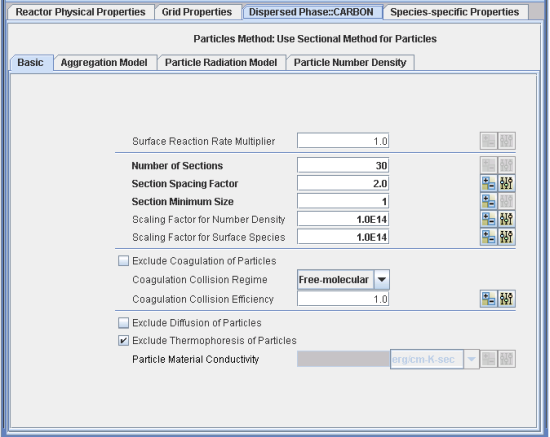
To consider a concrete example, as shown in Figure 19.1: Dispersed Phase panel to input parameters for sections. , the first section corresponds to particles with 1 monomer as given in the section minimum size (on the input panel). With a spacing factor of 2, the second section’s representative particle has 2 monomers, whereas the third section’s representative particle has 4 monomers, and so on. The section minimum size allows omission of sections with representative particles having fewer than a certain number of monomers. This can be useful, for example, when there is no particle depletion so that the minimum number of monomers in a particle is always greater than or equal to the monomers in a nucleation reaction.
If a spacing factor of less than 2 is used, some of the initial sections will have representative particles that cannot exist. For example, if the spacing factor in the previous example is 1.414, then the second section’s representative particle has 1.414 monomers in it and such a particle cannot physically exist. The solution of sectional model equations will return zero or a computationally negligible number for such sections as there will be no processes contributing to number density change in such sections. Note that although such spacing factors give sections corresponding to non-physical particles, it can be useful to resolve number density in larger size ranges.
It should be noted that the actual unknown that is solved for is the number density of the representative-size particles. The post-processor also gives dN /dLogD distribution as the experimental data is typically in this form. When writing this output it is assumed that the section volume boundaries are mid-way between the representative values. For the first and the last section, it is assumed that the representative volume is located mid-way between the bounding volumes. Thus, if there are 4 sections with representative volumes of 1, 2, 4, and 8 then the volume boundaries will be 0.5, 1.5, 3, 6, and 10. Since the actual number density data is available to the user, any other procedure could be used to compute dN /dLogD. Since the logarithm of diameter appears in the denominator, the partitioning used does not have a big influence.
A test matrix was applied to validate each component of the sectional model. Presented below are the results of two such tests.
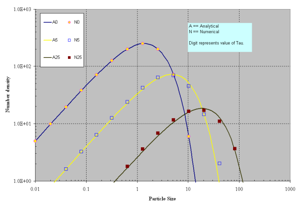
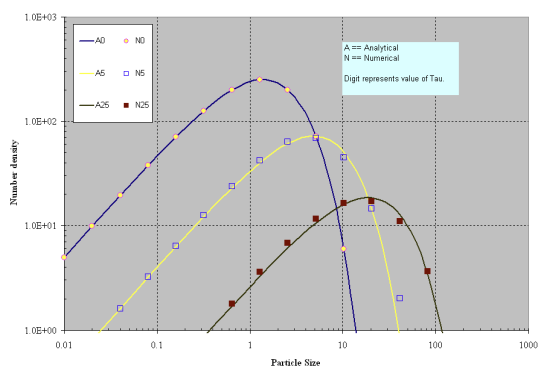
As mentioned earlier, only a handful of analytical solutions of the population-balance equation are available. For the case of an aggregation-only problem with a size-independent coagulation kernel with exponential initial distribution, the number density function is given as:
 | (19–18) |
 | (19–19) |
In the simulation results reported, the values of N 0 and β 8 are set to 1000 and 0.05, respectively. The minimum volume of the first section is set to V 0/100 and the volume (size) spacing follows V i +1 = 2*V i. The numerical solution computed using Equations Equation 19–14 to Equation 19–17 is plotted along with the analytical solution in Figure 19.2: Comparison of analytical and numerical solutions for exponential distribution. (Aggregation only, N 0 = 1000, β 0 = 0.05, plotted on linear scale for Y-axis). and Figure 19.3: Comparison of analytical and numerical solutions for exponential distribution. (Aggregation only, N 0 = 1000, B 0 = 0.05, plotted on logarithmic scale for Y-axis). . It can be seen in these figures that agreement is excellent.
Shown in Figure 19.4: Evolution of particle-size distribution for simultaneous nucleation and aggregation. are the results of simultaneous nucleation and agglomeration. The nucleation is assumed to happen in the first section and its rate is set to 1000*Exp(-t). The collision frequency is size-independent and is set to unity. At small values of t, the particle size distribution (PSD) is dominated by the nucleation. At moderate values of t a bimodal distribution is obtained. Although not shown in the figure, a similar PSD will evolve as in Figure 19.2: Comparison of analytical and numerical solutions for exponential distribution. (Aggregation only, N 0 = 1000, β 0 = 0.05, plotted on linear scale for Y-axis). when the nucleation rate becomes vanishingly small and only agglomeration takes place.
These results demonstrate that the initial implementation of the sectional model is working as expected for the Plug-Flow model. Future versions of the model will be extended to include the effects of growth and oxidation from surface chemistry.
Figure 19.2: Comparison of analytical and numerical solutions for exponential distribution. (Aggregation only, N 0 = 1000, β 0 = 0.05, plotted on linear scale for Y-axis).
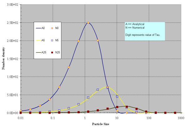
Figure 19.3: Comparison of analytical and numerical solutions for exponential distribution. (Aggregation only, N 0 = 1000, B 0 = 0.05, plotted on logarithmic scale for Y-axis).