


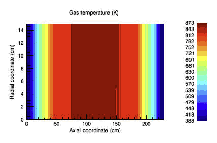
Figure 6.1: LPCVD Multiwafer Furnace-Gas Temperatures vs. Position shows a contour plot of the gas temperature as a function of radial and axial position in the reactor from the Ansys Chemkin Post-Processor. The gas temperatures are assumed to match the wall temperatures specified in the input temperature file, and show that the gas at the beginning and end of the reactor is significantly colder than the gas in the middle. The ends of these systems are generally not heated, as they often contain elastomeric materials used as vacuum seals. The surface temperatures in Figure 6.2: LPCVD Multiwafer Furnace-Surface Temperatures vs. Position show that the wafer temperatures also vary with axial distance, although the temperature range is much smaller. The end wafers are cooler as a result of radiative heat loss to the cooler ends of the reactor.

The contour plot of the silane mole fraction as a function of position in the reactor in Figure 6.3: LPCVD Multiwafer Furnace-Silane Mole Fractions vs. Position shows that the silane is significantly depleted as it flows downstream. This kind of depletion is generally compensated for by use of multiple injectors, or by imposing higher temperatures in the downstream portion of the reactor. The mole fraction at the end of the reactor is ~0.7, which means that most of the starting material passes through the system unreacted. In the radial direction, the profiles are fairly uniform, although there is some evidence of greater depletion in the center of the wafer load, as expected. Figure 6.4: LPCVD Multiwafer Furnace-Silylene Mole Fractions vs. Position shows that the silylene mole fraction is unevenly distributed in the reactor. This species is formed by decomposition of SiH4 in the gas phase, but also reacts very efficiently on the hot silicon surfaces. The highest mole fractions are therefore observed in the hot zones of the reactor away from the wafer load, where the ratio of surface area to volume is low.
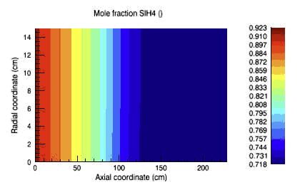
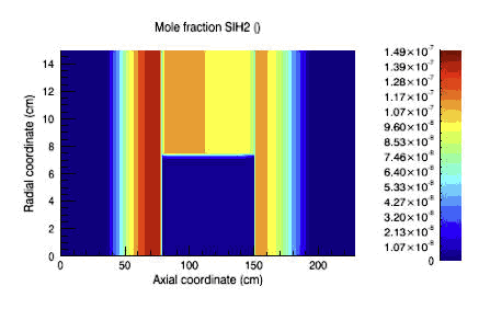
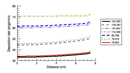
Figure 6.5: LPCVD Multiwafer Furnace-Deposition Rates on Wafers shows the deposition rate on the wafers as a function of axial position at the edge and center of the wafers, as well as the average value. Figure 6.6: LPCVD Multiwafer Furnace-Deposition Rates vs. Radial Position at Various Axial Positions shows a complementary plot of deposition rate as a function of radial position for the first three wafers, the center wafer, and the last three wafers in the reactor. The first few wafers and last few wafers have notably lower deposition rates as a result of being cooler than the rest. Measures of deposition uniformity down the load would normally not include the end wafer positions, where placeholder wafers are generally used. The deposition rate on the edge of the wafers is somewhat higher than at the center. The cross-wafer non-uniformity results both from temperature non-uniformity and from the SiH2 species, which is formed in higher concentration in the annular region between the wafers and the furnace wall, but then are depleted between the wafers by surface reactions.
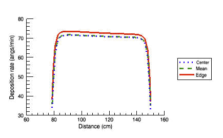
Figure 6.6: LPCVD Multiwafer Furnace-Deposition Rates vs. Radial Position at Various Axial Positions
In addition to the XML Solution File, the LPCVD Furnace model produces an output file that provides information about the run and numerical results. Generally, the user does not need to look at this file, but it does provide some numerical information that is not easily accessed from the graphical outputs. Also, if the simulation has difficulty finding a converged solution, error messages will be printed to this file. The sample output file can be found in the samples<release_number>\lpcvd_furnace\poly_si_deposition directory of the Ansys Chemkin installation after running the sample problem.
The output file first echoes back the Keyword inputs defining the model, then gives information about the grid that was built and the process of solving the model with the Ansys Chemkin two-point boundary-value solver, TWOPNT. In this case, the results from TWOPNT show that the solver starts with 50 time steps, unsuccessfully searches for the steady state, does another 50 time steps, then successfully finds the steady state. The output file then echoes back some keyword instructions, and lists results from the solution. For each axial grid point, it gives the position in cm, the axial gas velocity in cm/sec, the mole fractions for each gas species, the site fractions for each surface species, and the deposition rate in microns/min. The deposition rate is calculated from the molar production rate and the value of the bulk density for the bulk species as supplied in the SURFACE KINETICS input file. This deposition rate is for the outer wall of the reactor rather than an average over the wafer surfaces, as it includes regions of the reactor away from the wafer load. The file then gives the Atomic Element Budget, which in this case shows that only 16.395% of the silicon in the input stream gets incorporated into the deposited film. The file next gives a calculation of the deposition uniformity. The cross wafer percent uniformities given in the first two columns are for the best and worst wafer, which in this case are 2.372 and 15.170%, respectively (if the Annular Problem Only option is selected on the Reactor Geometry Properties panel, the output for these is 0.000). The third column gives the percent uniformity evaluated in the axial direction for all wafers in the load, which is the default. The rather large nonuniformity of 76.871% reported here reflects the fact that the deposition rates on the end wafers is much lower than the rest. Normally, these end wafers are not used, and the uniformity would be calculated over a smaller range of wafers specified by the user.
Detailed numerical results from the solution are also given in the plot files, 1d_gas.plt, 1d_surface.plt, 2d_gas.plt, and 2d_surface.plt. Examples of these files can be found in the samples<release_number>\lpcvd_furnace\poly_si_deposition directory of the Ansys Chemkin installation after running the sample problem. These files were originally formatted to be plotted with the Tecplot software, but are human-readable and could be used by other programs. The 1-D files give information on the axial dependencies of the variables. These files are most useful if the Annular Problem Only option is selected on the Reactor Geometry Properties panel to get radially averaged deposition rates. The 2-D files give both axial and radial dependencies, and provide detailed information on radial non-uniformities. In these files, the first line is a title line, which is followed by a list of the variables that are included in the file, such as axial or radial position, gas-phase mole fraction, surface site coverage, or deposition rates. This is followed by blocks of numbers giving the corresponding values, including also header comments identifying the variable and corresponding units.