The governing differential equations are made discrete using control volumes in the manner customary for reacting flow simulations. A differential conservation equation such as

(8–16)

in which is the quantity of the material conserved, is the material’s flux vector, and is the source, is equivalent to integral equations

(8–17)

for all "measurable" regions. With sufficient continuity and by Gauss' divergence theorem, the integral equation can be rewritten

(8–18)

in which is any sufficiently simple domain, is the domain's bounding surface, and is the surface's outward-pointing, unit normal vector [9].

The control volume approximation subdivides the domain of interest into a collection of (usually) polyhedral cells, 's, and then constructs an approximation to the integral equation, above, for each cell. The approximation arises because in evaluating the integrals

(8–19)

and are replaced by single values, and , uniformly distributed throughout the sub-domain, . Similarly, is replaced by a single vector throughout each polyhedral face. Moreover, if values for and are needed on a face, as when evaluating a diffusive flux, then those values must be approximated in some way from the cell values on either side. This process yields a collection of nondifferential (discrete) equations to be solved for the approximations, .

should approximate with increasing accuracy as all control volumes become smaller. Thus if computing resources permit, control volumes should be small.

The LPCVD Furnace Model's control volumes are determined by the radial and axial grids, with a typical control volume shown in Figure 8.1: A typical control volume . Faces determined by the axial grid slice the reactor tube into cylindrical pieces. In the region of the wafer load, faces determined by the radial grid further break these slices into rings. Figure 8.2: A control volume cross section with coordinates for grid points and boundaries is a detailed view of a cross-section through a control volume, showing how the cell faces are chosen to lie midway between grid points, so that the grid points lie strictly inside the resulting control volumes. Figure 8.3: Typical division of an LPCVD reactor into control volumes shows how a typical LPCVD reactor would be divided into control volumes. Details of grid determination are discussed in the next section.

Figure 8.1: A typical control volume

Figure 8.2: A control volume cross section with coordinates for grid points and boundaries

Figure 8.3: Typical division of an LPCVD reactor into control volumes

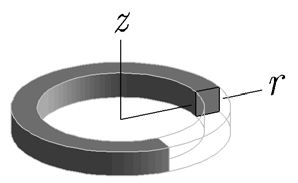
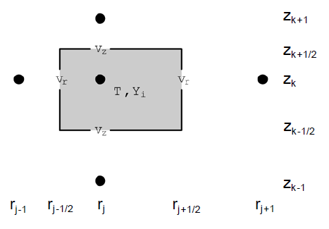
Figure 8.2: A control volume cross section with coordinates for grid points and boundaries also shows the relative positioning of the unknowns in the model. The unknown temperatures and mass fractions ( and ) in the LPCVD Furnace Model's equations are presumed to lie at the grid points, whereas the radial and axial velocities ( and ) are presumed to lie at the faces. Faces perpendicular to the radial axis have unknown but known ; faces perpendicular to the axial axis have known and unknown . This illustration is more general than actually occurs in the LPCVD Furnace Model. Due to the simplicity of the LPCVD Furnace Model's grid, gas may not flow through all four of the faces, in any control volume.

The overall discretization process is best illustrated by the equation for conservation of species mass. The LPCVD Furnace Model first replaces the differential equation (Equation 8–20 ) by an integral equation (Equation 8–21 ), and then approximates the integrals (Equation 8–22 ). Table 8.1: Approximate integrals for conservation of species mass equation shows the approximate integrals used in Equation 8–22 .

(8–20)

(8–21)

(8–22)

The subscripts in the approximate integrals index the locations shown in Figure 8.2: A control volume cross section with coordinates for grid points and boundaries . By convention, velocity is positive when in the direction of increasing or , so the signs in the boundary integral above vary with . Velocity at a cell face is a fundamental unknown, and is in either the axial or radial direction depending on the surface's orientation. For example, represents a radial velocity, . The LPCVD Furnace Model obtains other quantities at faces, such as density , by applying the appropriate subroutines to temperatures and mass fractions, and , averaged from the grid points on either side. The evaluation of diffusion velocities, , is therefore quite complicated. Factors in the approximate integrals such as and represent the following volumes and areas in Equation 8–23 through Equation 8–28 .

(8–23)

(8–24)

(8–25)

(8–26)

If a cell face coincides with a reacting surface, then the LPCVD Furnace Model does not make the substitution shown in Equation 8–27 that converts Equation 8–21 to Equation 8–22 . Instead, the terms in Equation 8–28 are used, representing flows to or from the surface.

(8–27)

(8–28)

All these terms have the same negative sign because the velocity, , in the boundary equation by convention points into the cell ( means the surface is a source of gas), which opposes the outward-pointing, unit normal vector, .

A major economy in the LPCVD Furnace Model's formulation is the ability to use one control volume to represent regions between several consecutive wafers. As illustrated in Figure 8.3: Typical division of an LPCVD reactor into control volumes , cells adjacent to injectors coincide with inter-wafer regions, while cells away from injectors span several inter-wafer regions. The approximate integral equations for these large cells lump their wafers’ reacting surfaces into just two surfaces. For purposes of printing, plotting and obtaining surface temperature data (from the TEMPERATURE FILE), the lumped surfaces lie at axially opposite sides of the large cells. This approximation is acceptable when, as is usually the case, deposition and temperature vary little among adjacent wafers.