Consider two phases , , which contain a component A, and consider the situation where the component A is in dynamic equilibrium between the phases. Typically, the concentrations of A in each phase are not the same. However, there is a well defined equilibrium curve relating the two concentrations at equilibrium. This is often, though not always, expressed in terms of mole fractions:

(5–233)

For binary mixtures, the equilibrium curve depends on temperature and pressure. For multicomponent mixtures, it also depends on mixture composition. The equilibrium curve is in general monotonic and nonlinear. Nevertheless, it is convenient to quasi-linearize the equilibrium relationship as follows:

(5–234)

Other useful forms of the equilibrium relationship are:

(5–235)

The various equilibrium ratios are related as follows:

(5–236)

 

5.13.3.1.1. Raoult’s Law

In gas-liquid systems, equilibrium relationships are most conveniently expressed in terms of the partial pressure of the solute in the gas phase.

It is well known that, for a pure liquid A in contact with a gas containing its vapor, dynamic equilibrium occurs when the partial pressure of the vapor A is equal to its saturated vapor pressure at the same temperature.

Raoult’s law generalizes this statement for the case of an ideal liquid mixture in contact with a gas. It states that the partial pressure of solute gas A is equal to the product of its saturated vapor pressure at the same temperature, and its mole fraction in the liquid solution .

(5–237)

If the gas phase is ideal, then Dalton’s law of partial pressures gives:

(5–238)

and Raoult’s law in terms of a mole fraction equilibrium ratio:

(5–239)

 

5.13.3.1.2. Henry’s Law

In the case of a gaseous material A dissolved in a non-ideal liquid phase, Raoult’s law must be generalized. Henry’s law states that a linear relationship exists between the mole fraction of A dissolved in the liquid and the partial pressure of A in the gas phase. This is:

(5–240)

is Henry’s constant for the component A in the liquid . It has units of pressure, and is known empirically for a wide range of material pairs, especially for common gases dissolved in water. It is strongly dependent on temperature.

Henry’s law may also be combined with Dalton’s law in order to express it in terms of a mole fraction equilibrium ratio:

(5–241)

Unfortunately, there is no common convention on the definition of Henry’s constant. Another definition in common use relates the partial pressure in the gas to the molar concentration in the liquid:

(5–242)

The two definitions of Henry’s constant are related by:

(5–243)

Due to the presence of discontinuities in concentration at phase equilibrium, it is, in general, not possible to model multicomponent mass transfer using a single overall mass transfer coefficient. Instead, it is necessary to consider a generalization of the Two Resistance Model previously discussed for heat transfer. For details, see The Two Resistance Model.

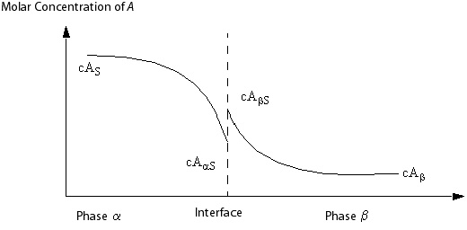
Consider a species A dissolved in two immiscible phases and . The basic assumption is that there is no resistance to mass transfer at the phase interface, and hence the equilibrium conditions prevail at the phase interface.

Also, it is assumed in this section that the total mass transfer due to species transfer is sufficiently small that primary mass sources to the phasic continuity equations are neglected. Hence, secondary mass fluxes to the species mass transfer equations are also ignored.

You model the component mass transfer using mass transfer coefficients , , defined on either side of the phase interface. These are usually defined so that driving forces are defined in terms of molar concentration differences. Thus, the molar flux of A to phase from the interface is:

(5–244)

and the molar flux of A to phase from the interface is:

(5–245)

Multiplying through by the molar mass of A, this determines the mass fluxes as follows:

Mass flux of A to phase from the interface:

Mass flux of A to phase from the interface:

(5–246)

In order to eliminate the unknown interface values, Equation 5–245 and Equation 5–246 must be supplemented by the equilibrium relation between and . This is most conveniently expressed using the molar concentration equilibrium ratio:

(5–247)

The mass balance condition:

(5–248)

may now be combined with the quasi-linearized equilibrium relationship Equation 5–247 to determine the interface mass concentrations:

(5–249)

These may be used to eliminate the interface values in Equation 5–245 and Equation 5–246 in order to express the interfacial mass fluxes in terms of the phasic mass concentrations:

(5–250)