The magnitude of the outlet velocity is specified and the direction is taken to be normal to the boundary at mesh resolution.

These are handled the same way as for an Inlet (Subsonic) boundary condition.
The Outlet Relative Static Pressure allows the pressure profile
at the outlet to vary based on upstream influences while constraining
the average pressure to a user-specified value  , where:
 | (1–229) |
where  is
the imposed pressure at each integration point and the integral is
evaluated over the entire outlet boundary surface. To enforce this
condition, the pressure at each boundary integration point is set
to:
is
the imposed pressure at each integration point and the integral is
evaluated over the entire outlet boundary surface. To enforce this
condition, the pressure at each boundary integration point is set
to:
 | (1–230) |
So, the integration point pressure in this case is set to the specified value plus the difference between the local nodal value and the average outlet boundary pressure. In this way the outlet pressure profile can vary, but the average value is constrained to the specified value.
In this case, the average pressure is only constrained in the region above or below the specified radius by shifting the calculated pressure profile by the difference between the specified average and the nodal average above or below the specified radius.
The circumferential averaging option divides the exit boundary condition into circumferential bands (oriented radially or axially depending on the geometry). The pressure within each band is constrained to the specified average pressure value the same way as is done for the overall averaging:
 | (1–231) |
where the specified value is applied within a band and the nodal average pressure is also calculated within a band.
The mass flux distribution across the outlet is determined by starting with the local mass flow rate distribution calculated by the flow solver at each integration point:
 | (1–232) |
From that distribution, you calculate the estimated total mass flow rate through the outlet boundary condition:
 | (1–233) |
where the summation is over all boundary integration points. A scaling factor is computed at the end of each coefficient loop that is used to scale the local integration point mass flows such that they add up to the specified mass flow rate:
 | (1–234) |
Iteratively, during the computation,  can be greater than
or less than unity. The final integration point mass flows are reset
by multiplying the integration point mass flows by the scaling factor:
can be greater than
or less than unity. The final integration point mass flows are reset
by multiplying the integration point mass flows by the scaling factor:
 | (1–235) |
In this way, the mass flux profile is an implicit result of the solution and at the same time gives exactly the specified mass flow rate.
This condition differs from the last one in that pressure is shifted in the continuity equation to get the specified mass flow rate. Generally speaking, the mass flow rate at each boundary integration point is dependent upon both velocity and pressure:
 | (1–236) |
where the integration point velocity depends upon nodal velocity and integration point pressures through the Rhie-Chow coupling. For this boundary condition, the integration point pressures are given by an expression of the form:
 | (1–237) |
where  is an optional
specified pressure profile,
is an optional
specified pressure profile,  is the boundary
node pressure,
is the boundary
node pressure,  is the outlet boundary nodal average pressure,
  is the Pressure Profile Blend factor that sets how much the specified
profile influences the boundary condition, and
is the Pressure Profile Blend factor that sets how much the specified
profile influences the boundary condition, and  is the level shift factor automatically computed
by the CFX-Solver each coefficient loop to enforce the specified mass
flow rate, such that:
is the level shift factor automatically computed
by the CFX-Solver each coefficient loop to enforce the specified mass
flow rate, such that:
 | (1–238) |
where the sum, in this case, is over all the outlet boundary condition integration points.
A further extension of the shift pressure feature for outlet mass flow rate conditions (or outlet boundaries using an Average Static Pressure specification) enforces the specified profile as an average pressure profile (or average pressure) in circumferential bands (radial or axial), held at a particular value.
Starting with the original formula for the integration point pressure in Equation 1–237: instead of imposing a particular profile distribution, an average pressure profile within bands is introduced:
 | (1–239) |
where:  is the average pressure desired in band
  , and
, and  is the current average nodal value
in band
is the current average nodal value
in band  .
.  corresponds
to the Pressure Profile Blend factor. When
the specified profile spatially varies, the flow solver will compute
the average of that profile within each band and then use those
values for
corresponds
to the Pressure Profile Blend factor. When
the specified profile spatially varies, the flow solver will compute
the average of that profile within each band and then use those
values for  .
.
The Exit Corrected Mass Flow Rate (ECMF) boundary condition allows you to specify an equivalent mass flow rate corrected to a user specified reference temperature and pressure. If the reference conditions are not provided, reference conditions will default to 1 [atm] and 15 [°C], corresponding to Standard Atmosphere Sea Level Static conditions.
Performance of compressible turbomachinery is generally dependent on ten variables; blade tip diameter, rotational speed, mass flow rate, inlet total temperature and pressure, exit total temperature and pressure, gas constant, specific heat ratio, and viscosity. These ten variables may be reduced to six similarity criteria: pressure ratio, temperature ratio, non-dimensional mass flow, non-dimensional speed, Reynolds number, and the ratio of specific heats.
The non-dimensional mass flow parameter ( ) is taken as the ratio of
the actual mass flow rate to that which would pass through an orifice
of diameter
) is taken as the ratio of
the actual mass flow rate to that which would pass through an orifice
of diameter  with a velocity equal to the stagnation speed of sound.
 | (1–240) |
where  and
and  are the stagnation (total)
density and speed of sound at the outlet, respectively. The ECMF is
obtained by multiplying the non-dimensional mass flow by a constant
value equal to the mass that would pass through an orifice of the
same diameter,
are the stagnation (total)
density and speed of sound at the outlet, respectively. The ECMF is
obtained by multiplying the non-dimensional mass flow by a constant
value equal to the mass that would pass through an orifice of the
same diameter,  , at a speed equal to the speed of sound at reference conditions.
 | (1–241) |
For ideal gases, we can substitute  and
and  with:
with:


at the local and reference conditions, where  is the ratio of specific
heats and
is the ratio of specific
heats and  is the specific gas constant.
This reduces Equation 1–241to:
 | (1–242) |
where  and
and  are the stationary
frame total pressure and total temperature at the outlet.
are the stationary
frame total pressure and total temperature at the outlet.
To obtain a mass flow at the boundary, Equation 1–242is rearranged to obtain the actual mass flow rate based on the current outlet conditions and the specified corrected mass flow, written as:
 | (1–243) |
where,  and
and  are mass averaged values of total pressure and temperature
in the stationary frame at the outlet.
are mass averaged values of total pressure and temperature
in the stationary frame at the outlet.
Note that the current implementation is based on the ideal gas
reduction above. While the boundary condition will still provide the
stability benefits for non-ideal gas simulations, the specified corrected
mass flow may not correspond exactly to Equation 1–241due to differences in how  and
and  are computed from the equation of state.
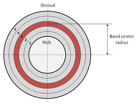
The radial equilibrium option divides the boundary condition into radially oriented circumferential bands. The pressure within each band is constrained by the radial equilibrium condition:
 | (1–244) |
This equation is used to calculate the pressure gradient  in each band,
  , based on the band
averaged tangential velocity,
, based on the band
averaged tangential velocity,  , and density,
  , as well as the band center
radius,
, as well as the band center
radius,  . The band edge pressures,
  , are obtained by
integrating this equation starting from the specified pressure at
the radial reference position. This pressure is used to constrain
the solution pressure with the following equation:
, are obtained by
integrating this equation starting from the specified pressure at
the radial reference position. This pressure is used to constrain
the solution pressure with the following equation:
 | (1–245) |
where:
 is the area average nodal pressure, within
a band
is the area average nodal pressure, within
a band 
 is linearly interpolated between
the band edge values to the local face radius, r
is linearly interpolated between
the band edge values to the local face radius, r
and
 is the evaluated pressure at the band mid-radius.
As for all average static-pressure options, the pressure profile
blend factor, F, can be applied to this boundary
condition. If the factor F=,1 then the pressure
at each face is fully constrained to the pressure obtained from the
radial equilibrium condition,  , so that a circumferential profile
is not allowed within the band. If the factor F=0, then a circumferential profile is allowed to develop with the
average of that profile equal to the radial equilibrium pressure.
, so that a circumferential profile
is not allowed within the band. If the factor F=0, then a circumferential profile is allowed to develop with the
average of that profile equal to the radial equilibrium pressure.