


The equilibrium phase change model is a single fluid, multicomponent phase change model. The model is especially suitable for flows of condensing vapors (for example, wet steam or refrigerants) with small liquid mass fractions but it can also be used for some melting or solidification problems as well.
This model assumes that the mixture of the two phases is in local thermodynamic equilibrium. This means that the two phases have the same temperature and that the phase change occurs very rapidly, such that the mass fractions may be determined directly from the phase diagram.
In addition to the superheat region, the equilibrium phase change model requires knowledge of the phase diagram of the material being modeled. Consider Figure 12.6: Phase Diagram, which shows two lines of constant pressure that go through the saturation dome on a temperature-entropy diagram for a vapor-liquid mixture.
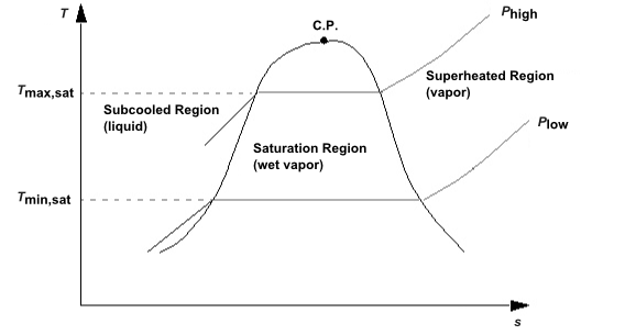
To the left of the dome, the entropy is lower than the saturation entropy of the liquid, and the mixture is all liquid. To the right, the entropy is greater than the saturation entropy of the vapor, and the mixture is all vapor. In the remaining region, underneath the saturation dome, the mixture contains both liquid and vapor.
To determine the mass fraction of the vapor, or quality ( ), the flow solver uses
the lever rule:
), the flow solver uses
the lever rule:
 | (12–2) |
where  is the mixture static
enthalpy calculated by the flow solver (either directly or from total enthalpy), and
is the mixture static
enthalpy calculated by the flow solver (either directly or from total enthalpy), and
 and
and  are the saturation enthalpies of the liquid and vapor respectively as
a function of pressure. The following observations can be made about the quality:
are the saturation enthalpies of the liquid and vapor respectively as
a function of pressure. The following observations can be made about the quality:
When
 , the mixture is 100% subcooled liquid so
the liquid properties are selected.
, the mixture is 100% subcooled liquid so
the liquid properties are selected.When
 , the mixture is 100% superheated vapor so
the vapor properties are selected.
, the mixture is 100% superheated vapor so
the vapor properties are selected. When
 , the mixture contains liquid and
vapor. The bulk mixture properties are calculated using the lever rule. Using
the mass fraction of vapor and the saturated liquid and vapor properties this
gives:
, the mixture contains liquid and
vapor. The bulk mixture properties are calculated using the lever rule. Using
the mass fraction of vapor and the saturated liquid and vapor properties this
gives:
(12–3)
where  is a property such as entropy, enthalpy,
specific heat, thermal conductivity or dynamic viscosity. Because density is volumetric,
saturated density is calculated using harmonic averaging instead:
is a property such as entropy, enthalpy,
specific heat, thermal conductivity or dynamic viscosity. Because density is volumetric,
saturated density is calculated using harmonic averaging instead:
 | (12–4) |
Derivatives of density with respect to pressure along the saturation line are derived from the harmonic average expression using the chain rule:
 | (12–5) |
where we have not yet decided which variable,  , is held constant. If
the densities are a function of pressure, which they usually are, expressions for the
speed of sound can be derived using Equation 12–5,
and the standard thermodynamic relationship:
, is held constant. If
the densities are a function of pressure, which they usually are, expressions for the
speed of sound can be derived using Equation 12–5,
and the standard thermodynamic relationship:
 | (12–6) |
For the purposes of the equilibrium phase change model the isentropic speed of sound is output as the variable "Local Speed of Sound" and is computed as follows:
 | (12–7) |
substituting Equation 12–5 held at constant temperature. The mixture specific heat capacities are evaluated using Equation 12–3. Equation 12–7 is applied in all regions, however, the mixing rule for the isothermal derivative, Equation 12–5, is only applied in regions where the equilibrium fraction is non-zero or unity.
While the formulas just presented assume that you are modeling a mixture of liquid and vapor, the same algorithm also holds for other types of phase change, such as the melting and solidification of solid and liquid water, respectively.