


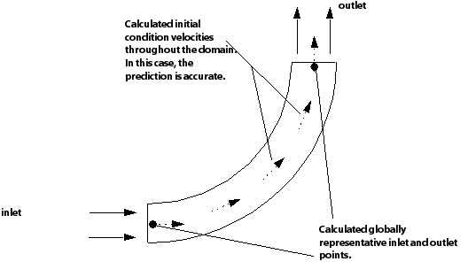
For Automatic Values, the initial conditions are based on a linear evaluation. Evaluation of linear initial conditions requires two points in the solution domain and initial condition values at these points. These points and initial condition values are generated using a weighted average of boundary condition information from all inlets, openings and outlets. The two points may be considered as a globally representative inlet and outlet. For example, the first point (the globally representative inlet) is located at an average of the centroids of all inlet, opening and outlet boundaries where the inlet boundary information is weighted much more heavily than the information from other boundaries. The initial condition value(s) for this point are similarly evaluated. See Figure 3.1: Initial Condition Values for an illustration.
The direction and magnitude of velocity linear initial conditions are treated independently. This reflects the use of velocity-specified (the direction and magnitude specified) boundary conditions, and of direction-specified (the total pressure and normal direction) boundary conditions.
When direction information is available from boundary conditions, it is used. If no information is available, a boundary normal direction is assumed. Note that zero vectors are possible for the globally representative inlet and outlet direction vectors because of the direction averaging (for example, two similar inlets that face each other).
Magnitude information is similarly used when it is available from the boundary conditions (note that an approximate velocity is calculated for mass flow specified boundary conditions). If no velocity magnitude information is available from boundary conditions (such as total pressure inlet, static pressure outlet), then half of the average rotational velocity (that is, the angular velocity multiplied by the mean radius) over a given boundary is used. This gives a reasonable "velocity triangle" approximation for turbo machines, and results in a magnitude of zero for stationary domains.
Note that the linear initial condition reverts to a constant velocity magnitude (or pressure) if only one value can be derived from boundary condition information (for example, constant pressure for total pressure in, mass flow out).
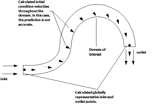
Important: When applying initial conditions, the shape of your domain(s) is an important consideration when applying an automatic initial guess. As Figure 3.2: Inaccurate Initial Conditions shows, a linearly varying prediction for velocity is not always appropriate. You can disable the automatic initial guess for velocity by setting the velocity scale to 0 m/s. For details, see Velocity Scale.
If you suspect that the flow is predominantly in a particular direction through the domain (for example, in the direction of an Inlet specification), you can initialize the velocity components to this direction. You should not set a velocity higher than the inlet velocity.
If you predict that the Automatic method is unsuitable
for your simulation, but do not want to specify Cartesian components, setting
the velocity scale to zero imposes a zero velocity field throughout the domain.
For details, see Velocity Scale.
An explanation of how coordinate frames interact with velocity components is available in Coordinate Frame.
Information on modeling multiphase flow is available in Initial Conditions for a Multiphase Simulation.