


When you use a cubic equation of state for a dry vapor calculation or for non-equilibrium phase change calculations (using the thermal phase change model or small droplet phase change model), the flow solver enables the vapor and liquid states to go inside the saturation dome locally. The properties are clipped at the vapor or liquid spinodal curve. The spinodal curve defines the boundary beyond which the equation of state is no longer valid because the local derivative of pressure with respect to volume becomes positive. State points predicted inside the dome, up to the spinodal curve, are called "metastable" because normally they only exist temporarily in small local regions until phase change occurs.
For example, metastable states may occur during the calculation when the vapor cools below the local saturation temperature due to rapid flow expansion (called supercooling) or the liquid temperature locally rises above saturation due to rapid heating or compression (called superheating). For cases without phase change these states can occur and continue to persist depending on the problem set-up.
As an example, Figure 12.1: Pressure Volume Diagram for Water (Peng Robinson Equation of State), and Figure 12.3: Vapour Pressure Diagram for Water (Peng Robinson Equation of State) illustrate what the spinodal curves look like on a pressure-volume diagram and pressure-temperature diagram for water when using the Peng Robinson equation of state. Figure 12.2: Pressure Volume Diagram for Water (Aungier Redlich Kwong Equation of State) and Figure 12.4: Vapour Pressure Diagram for Water (Aungier Redlich Kwong Equation of State) show the curves that are obtained when the Aungier Redlich Kwong equation of state is used.
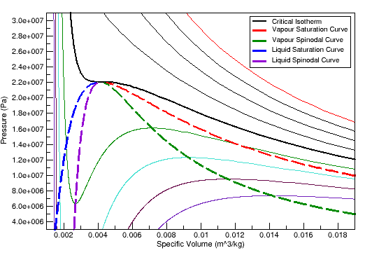
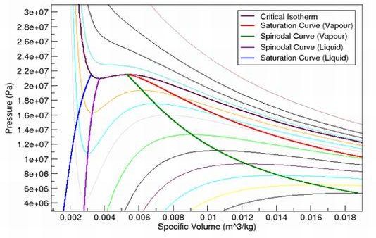
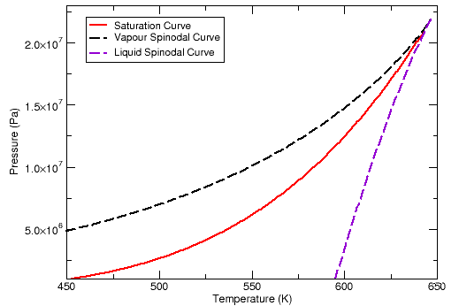
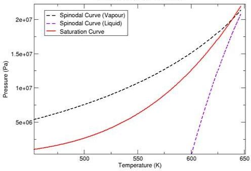
As you can see, the spinodal states for water vapor enable the vapor to cool below the saturation temperature, and similarly for liquid water heat above the saturation temperature. Normally, though, these states do not remain stable for long before phase change happens.
When you run an equilibrium phase change calculation, it is not necessary to predict metastable states inside the saturation dome, so the vapor and liquid properties are clipped at the saturation curve instead of the spinodal curves.
The spinodal curves are derived directly from the equation of state by finding
where  . The vapor pressure
curve can be derived from a general equation of state by Gibbs energy minimization.
However, to reduce computational cost, the cubic equation of state models assume the
saturation curve is given by an equation from Poling et al. [84]:
. The vapor pressure
curve can be derived from a general equation of state by Gibbs energy minimization.
However, to reduce computational cost, the cubic equation of state models assume the
saturation curve is given by an equation from Poling et al. [84]:
 | (12–1) |
where  is the acentric factor. The acentric
factor is a property of a pure fluid and is tabulated in many different
thermodynamics references (see, for example, [84]).This equation accurately predicts the saturation curve
for most cubic equations of state. If the acentric factor is not tabulated it can
easily be estimated using an alternative form of the vapor pressure curve (for
example, the Antoine equation) and the following equation:
is the acentric factor. The acentric
factor is a property of a pure fluid and is tabulated in many different
thermodynamics references (see, for example, [84]).This equation accurately predicts the saturation curve
for most cubic equations of state. If the acentric factor is not tabulated it can
easily be estimated using an alternative form of the vapor pressure curve (for
example, the Antoine equation) and the following equation:

where  is the critical pressure and
the vapor pressure,
is the critical pressure and
the vapor pressure,  , is evaluated from the
Antoine equation, with the temperature set equal to
, is evaluated from the
Antoine equation, with the temperature set equal to  .
However, using the Antoine equation also requires that the Antoine coefficients be
known.
.
However, using the Antoine equation also requires that the Antoine coefficients be
known.