


For transient simulations with Lagrangian particles, it is very helpful to define integrated quantities:
The axial penetration of a spray measured along the user-defined spray axis (SA in Figure 8.8: Spray Penetration)
The radial penetration of a spray measured normal to the user-defined spray axis (SR in Figure 8.8: Spray Penetration)
The penetration of a spray normal to the spray axis (SN in Figure 8.8: Spray Penetration)
The penetration angle of a spray (
 in
Figure 8.8: Spray Penetration)
in
Figure 8.8: Spray Penetration)The total mass of particles
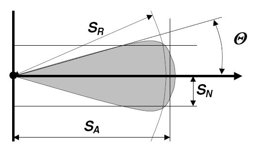
The penetration is normally evaluated by looking at a specified fraction of the spray, that is, the axial penetration of a spray is given by a distance from the spray nozzle that contains 99 percent of the particle mass. The calculation of the axial, radial, and normal penetration depth is straightforward.
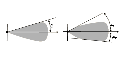
The spray angle as reported by the transient particle diagnostics is calculated as
follows: An imaginary cone is created with its tip at the point of injection and the
cone axis parallel to the specified injection direction. The cone angle is then
gradually increased up to the point where the imaginary cone contains a certain
percentage of the total spray mass (by default: 99%, this can be changed via the
Contained Spray Mass Fraction CCL parameter). The cone half
angle is then reported as the spray angle,  .
.
Figure 8.9: Spray Angle Calculation for Different Spray Shapes shows two typical spray shapes and the reported spray
angle,  .
.
When the spray is injected with a finite injection radius as shown in Figure 8.10: Spray Angle Calculation with Finite Injection Radius with and without Spray
Radius Specified, you will need to set the Spray Radius at
Penetration Origin parameter to the size of the injection radius,
otherwise the solver will return a spray angle of 90°.
Figure 8.10: Spray Angle Calculation with Finite Injection Radius with and without Spray Radius Specified

There are various different ways to calculate transient particle diagnostics. A flexible User Fortran interface is available that enables you to calculate any information from all particles (given by their position, velocity, …) at any time step during a transient particle run.
Besides the hard coded penetration depth and angle it is necessary to provide a method that enables you to evaluate any transient particle diagnostics. You cannot use CEL expressions for particles. As an alternative, it is possible to call a user routine that evaluates the required diagnostics information based on a specified list of particle variables. The following particle variables can be chosen:
Mean Particle NumberParticle Number RateParticle PositionParticle TimeParticle Traveling DistanceTemperatureTotal Particle MassVelocity
Following this approach, the solver provides the values of all particle variables specified for user-defined diagnostics in a local working directory, together with global information about the total number of particles (NPART) at the current time step, as well as the particle type (CPT) and particle type alias name (ALIAS). This is necessary because user routines do not support subroutine arguments besides the five Fortran stacks. The user routine can now pick up the required information from the MMS by converting the variable names specified to internal solver names for which standard LOCDAT calls can be used. The obtained pointers can be passed down to another subroutine layer, which does the final calculation.
In order to monitor values calculated within the user routine, you can store a defined list of REAL variables back to the MMS (predefined place is TPD_VALUE in the local directory). Those variables are picked up by the solver and are written to the CFX-Solver Output file similar to the pre-defined transient diagnostics values. The values are also added to the list of monitored values for the Ansys CFX-Solver Manager. You must specify a list of strings (CCL-parameter: Monitored Values List) which contains names for the values to be monitored. The number of monitored values is determined from this list and the names are used in the CFX-Solver Output file and in the CFX-Solver Manager.
As an example for this strategy, a user routine has been created that simply calculates the particle mass within three spheres with different user-specified radii. The next subsections show the CCL and the listings of the required user routine, as well as the diagnostics output.
Sphere radius and center is specified in the USER section of the CCL:
USER: CENTRE = 0.5, 0.5, 0.5 RADIUS1 = 0.25 RADIUS2 = 0.35 RADIUS3 = 0.45 END
The CCL definition for the corresponding junction box is as follows:
TRANSIENT PARTICLE DIAGNOSTICS: User Routine Sphere
Option = User Defined
Transient Particle Diagnostics Routine = Sphere
Particle Variables List = \
Particle Position, \
Total Particle Mass, \
Particle Number Rate
Monitored Values List = \
First sphere, \
Second sphere, \
Third sphere
Particles List = Water
END
As can be seen, the user routine depends on the position, mass, as well as the number rate of the particles and provides three values that are monitored during the simulation. The new diagnostics section for this CCL in the CFX-Solver Output file looks like:
+--------------------------------------------------------------------+
| Transient Particle Diagnostics |
+--------------------------------------------------------------------+
Water
User Routine Sphere
First sphere 3.8847E-02
Second sphere 5.9132E-02
Third sphere 7.2068E-02
In the
<install_dir>\examples\UserFortran
directory, you can find an example mainline routine,
pt_tpd1.F, and corresponding CCL template,
pt_tpd1.ccl.
SUBROUTINE CALC_TPD1(TOTAL_MASS,SPHERE_CENTRE,
& SPHERE_RADIUS,NPART,CRD,MASST,RATE)
C
C=======================================================================
C Subroutine for CALC_TPD1 which does the real calculation
C=======================================================================
C
INTEGER NPART
REAL TOTAL_MASS(3), SPHERE_CENTRE(3), SPHERE_RADIUS(3),
& CRD(3,NPART), MASST(NPART), RATE(NPART)
C
INTEGER IPART, I
REAL RADIUS
C
DO I=1,3
TOTAL_MASS(I) = 0.0
ENDDO
C
DO IPART=1,NPART
RADIUS = SQRT( (CRD(1,IPART)-SPHERE_CENTRE(1))**2
& + (CRD(2,IPART)-SPHERE_CENTRE(2))**2
& + (CRD(3,IPART)-SPHERE_CENTRE(3))**2 )
DO I=1,3
IF (RADIUS.LE.SPHERE_RADIUS(I)) THEN
TOTAL_MASS(I) = TOTAL_MASS(I) + MASST(IPART)*RATE(IPART)
ENDIF
ENDDO
ENDDO
C
END
The following CCL for
Two penetration objects
Specified location
Specified particle injection region (PIR)
One total particle mass object
Two user defined diagnostics objects
User routine with three monitored values
User routine without any monitored values
looks as follows:
#=======================================================================
# TRANSIENT PARTICLE DIAGNOSTICS
#=======================================================================
#
#-----------------------------------------------------------------------
# Penetration
#-----------------------------------------------------------------------
#
TRANSIENT PARTICLE DIAGNOSTICS: Penetration from Location
Option = Particle Penetration
PENETRATION ORIGIN AND DIRECTION:
Option = Specified Origin and Direction
Injection Centre = 0.01 [m], 0.5 [m], 0.01 [m]
INJECTION DIRECTION:
Injection Direction X Component = 1.0
Injection Direction Y Component = 0.0
Injection Direction Z Component = 1.0
Option = Cartesian Components
END
END
Contained Spray Mass Fraction = 0.98
Particles List = Water 1
AXIAL PENETRATION:
Option = Axial Penetration
END
RADIAL PENETRATION:
Option = Radial Penetration
END
NORMAL PENETRATION:
Option = Normal Penetration
END
SPRAY ANGLE:
Option = Spray Angle
END
END
TRANSIENT PARTICLE DIAGNOSTICS: Penetration from PIR
Option = Particle Penetration
PENETRATION ORIGIN AND DIRECTION:
Option = Particle Injection Region
Particle Injection Region = Cone
END
Contained Spray Mass Fraction = 0.98
Particles List = Water 1, Water 2
AXIAL PENETRATION:
Option = Axial Penetration
END
RADIAL PENETRATION:
Option = Radial Penetration
END
NORMAL PENETRATION:
Option = Normal Penetration
END
SPRAY ANGLE:
Option = Spray Angle
Spray Radius at Penetration Origin = 0.005 [m]
END
END
#
#-----------------------------------------------------------------------
# Total Particle Mass
#-----------------------------------------------------------------------
#
TRANSIENT PARTICLE DIAGNOSTICS: Total Particle Mass
Option = Total Particle Mass
Particles List = Water 1, Water 2
END
#
#-----------------------------------------------------------------------
# User Defined
#-----------------------------------------------------------------------
#
TRANSIENT PARTICLE DIAGNOSTICS: User Routine Sphere
Option = User Defined
Transient Particle Diagnostics Routine = Sphere
Particle Variables List = \
Particle Position, \
Total Particle Mass, \
Particle Number Rate
Monitored Values List = \
First sphere, \
Second sphere, \
Third sphere
Particles List = Water 1, Water 2
END
TRANSIENT PARTICLE DIAGNOSTICS: User Routine Histo
Option = User Defined
Transient Particle Diagnostics Routine = Histogram
Particle Variables List = \
Total Particle Mass, \
Particle Number Rate, \
Mean Particle Diameter
Particles List = Water 1, Water 2
END
Leading to the following lines in the CFX-Solver Output file and in the CFX-Solver Manager:
+--------------------------------------------------------------------+
|                     Transient Particle Diagnostics                 |
+--------------------------------------------------------------------+
Water 1

   User Routine Histo
   User Routine Sphere
      First sphere                           3.8847E-02
      Second sphere                          5.9132E-02
      Third sphere                           7.2068E-02
   Total Particle Mass
      Total Particle Mass                    1.0000E-01
   Penetration from PIR
      Axial Penetration                      7.7220E-01
      Radial Penetration                     8.0765E-01
      Normal Penetration                     2.4617E-01
      Spray Angle                            3.9586E+01
   Penetration from Location
      Axial Penetration                      7.7220E-01
      Radial Penetration                     8.0765E-01
      Normal Penetration                     2.4617E-01
      Spray Angle                            4.6757E+01

Water 2

   User Routine Histo
   User Routine Sphere
      First sphere                           4.5829E-02
      Second sphere                          6.1053E-02
      Third sphere                           7.3941E-02
   Total Particle Mass
      Total Particle Mass                    1.0000E-01
   Penetration from PIR
      Axial Penetration                      7.8456E-01
      Radial Penetration                     9.6701E-01
      Normal Penetration                     6.7314E-01
      Spray Angle                            8.7652E+01
You can use the Particle Histogram option under the
Particles tab of Output Control to
define particle histogram data of track variables on user-specified boundary
patches and/or particle injection regions. For details, see Particle Histogram in the CFX-Pre User's Guide.
You can also use the Particle Track Data option under the
Export Results tab in Output
Control to export a specified list of particle data on specified
boundaries or particle injection regions. For details, see Particles Tab in the CFX-Pre User's Guide.