


CFX offers two kinds of mass/momentum modeling options at domain interfaces: a user-specified pressure change and a user-specified mass flow rate. These have different applications depending on the type of domain interface.
It is often useful to model periodic flow but enable a pressure drop between the two sides of the interface. Examples of this include:
flow through tube banks in heat exchangers
periodic duct flow
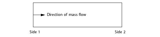
If the pressure drop is specified, the solver will calculate the flow field including the mass flow rate. Alternatively, if the mass flow rate through the interface is known, the solver will calculate the flow field including the pressure drop. If a pressure change condition is specified, the specified pressure change is assumed to be from side 1 to side 2 of the interface (see the figure below). For pressure drop situations like flow through a duct or tube bank, this pressure change should be negative. If a mass flow rate condition is specified, the specified mass flow rate is assumed to be into the domain through side 1 and out of the domain through side 2.
The following sections describe applying a specified pressure change or a mass flow rate to a general domain interface.
It is sometimes useful to apply a pressure change condition to a general domain interface. For example, a screen model might prescribe a pressure drop at the domain interface which is proportional to the local dynamic head:
 | (5–1) |
where  is the screen loss coefficient
and
is the screen loss coefficient
and  is the pressure change measured from side 1 to side 2. This screen model can
be implemented using the following CEL expression:
is the pressure change measured from side 1 to side 2. This screen model can
be implemented using the following CEL expression:
Pressure Change = -k * density * (u^2 + v^2 +
w^2)
Note that in the case that the density in the above expression is itself dependent on the pressure, such as for an ideal gas, the pressure from side 2 is used to evaluate the density.
Another application of the pressure change condition is modeling a fan for which the pressure rise is a function of the mass flow rate:
 | (5–2) |
This fan model can be implemented by creating an interpolation function or
CEL expression for  ;
for example, if one side of the domain interface has the name
;
for example, if one side of the domain interface has the name Fan
Side 1, one could create a CEL expression or interpolation
function for  as follows:
Pressure Change=f(massFlow()@Fan Side 1)
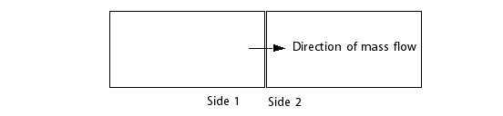
The mass flow rate can also be specified through a general connection. The specified mass flow rate is assumed to be from side 1 to side 2 of the interface. See the figure below.
The solver implements the specified mass flow condition by adjusting the pressure change until the specified mass flow rate is satisfied. Prior to convergence, the actual mass flow rate may not satisfy the specified mass flow rate, although it typically becomes close within a few dozen iterations. To enhance robustness of this condition, the pressure change is under-relaxed with a default under-relaxation factor of 0.25. This value can be increased if convergence to the specified mass flow rate is slow but monotonic and decreased if convergence to the specified mass flow rate is oscillatory or unstable.
When using a pressure change, the solver checks an additional criterion when deciding whether the problem has converged. For the pressure change condition, the solver checks whether
 | (5–3) |
where  is the domain
interface convergence criterion. By default,
is the domain
interface convergence criterion. By default,  is 0.01, but can
be modified by changing Domain Interface Target on the
Solver Control tab in CFX-Pre.
is 0.01, but can
be modified by changing Domain Interface Target on the
Solver Control tab in CFX-Pre.
When using a mass flow rate condition, the solver checks the following additional criterion when deciding whether the problem has converged:
 | (5–4) |
The mass flow rate through each side of the domain interface can be monitored
by creating a new plot in the CFX-Solver Manager. For the plot line, select
FLOW, then DOMAIN INTERFACE, then
the domain interface side you want to monitor, and then choose
P-Mass.