


This section provides a brief description of the linear regular wave (Airy wave) and the second order Stokes wave in either deep water or finite depth water.
Linear wave (Airy wave) is considered as the simplest ocean wave, and is based on the assumption of homogeneous, incompressible, inviscid fluid and irrotational flow. In addition, the wave amplitude is assumed to be small compared to the wave length and water depth; hence the linear free surface condition is used.
In the fixed reference axes (FRA), the water surface elevation at position X and Y can be expressed in complex value form as
 | (2–1) |
where  is the wave amplitude,
  is the wave frequency (in rad/s),
  is the wave number,
  is the wave propagating
direction, and
is the wave propagating
direction, and  is the wave phase.
Assuming ideal, irrotational fluid, the flow can be represented by a velocity potential satisfying the Laplace equation in the whole fluid domain, the linear free surface condition, and horizontal impermeable bottom condition.
In finite depth water, the velocity potential at the location
of  is
is
 | (2–2) |
where  is water depth and
  is gravitational acceleration.
Employing the linear free surface condition, the relationship between the wave frequency and the wave number (the linear dispersion relationship) is represented by
 | (2–3) |
The wave length and wave period are
 | (2–4) |
Using the Bernoulli equation and only taking account the linear term, the fluid pressure is
 | (2–5) |
where  is the water density.
The wave celerity is
 | (2–6) |
Taking the partial derivative of the velocity potential, the fluid particle velocity is
 | (2–7) |
When the wave particle velocity at the crest equals the wave celerity, the wave becomes unstable and begins to break (see [39]). The limiting condition for wave breaking in any water depth is given by:
 | (2–8) |
In infinite depth water ( ), the wave elevation keeps the same form as Equation 2–1, but velocity potential is further simplified
as
), the wave elevation keeps the same form as Equation 2–1, but velocity potential is further simplified
as
 | (2–9) |
the linear dispersion relation is expressed as
 | (2–10) |
and the fluid pressure is
 | (2–11) |
the wave celerity and fluid particle velocity are expressed as
 | (2–12) |
From Equation 2–8, for deep water wave,
the wave breaks when the wave height ( ) is 1/7th of
the wave length.
) is 1/7th of
the wave length.
Advanced wave theories may be necessary in some cases when the nonlinearities are important (see [4] and [8]). Aqwa allows application of the second order Stokes wave theory for moderate or severe regular wave conditions when the nonlinear Froude-Krylov force over the instantaneous wetted surface is estimated.
Choosing the ratio of the wave amplitude to wave length as the
smallness parameter  , Taylor expansions for the velocity potential
and wave surface elevation in
, Taylor expansions for the velocity potential
and wave surface elevation in  can be written as
 | (2–13) |
For water of finite depth, the second order Stokes wave is expressed as
 | (2–14) |
where  .
.
When the set-down in the second-order Stokes waves is included, the potential and wave elevation are written as
 | (2–15) |
where

The above new terms are negative constants called set-down, which represent the mean level in regular Stokes waves.
The velocity of a fluid particle at coordinates (X, Y, Z) is
 | (2–16) |
The fluid pressure up to the second order is
 | (2–17) |
Comparing with the linear Airy wave, the second order Stokes wave profile shows higher peaked crests and shallower, flatter troughs.
For deep water cases ( ), the second order Stokes wave given in Equation 2–15 becomes
 | (2–18) |
Note that in deep water, the second order Stokes wave potential only consists of the first order components, and there is no set-down term.
Aqwa allows the application of the fifth order Stokes wave theory for moderate or severe regular wave conditions when the nonlinear Froude-Krylov force over the instantaneous wetted surface is estimated.
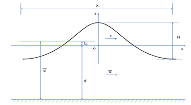
The fifth order Stokes wave solution developed by Zhao, et al. [45] is employed. The solution is represented in the wave fixed
reference coordinate system, of which the origin is on the undisturbed water surface, the
x-axis is along the wave propagation direction, and the z-axis is upwards. The time equals zero
when the wave crest passes through the origin of this coordinate system. Figure 2.1: Fifth Order Stokes Wave shows one cycle wave sketch and some important quantities, i.e.
c as the wave celerity,  as the uniform current along the wave propagation direction,
d as the still water depth,
as the uniform current along the wave propagation direction,
d as the still water depth,  as the mean water depth that is wave dependent, and H as
the crest-to-trough wave height.
as the mean water depth that is wave dependent, and H as
the crest-to-trough wave height.
Denoting  as the wave direction in the fixed reference axes of OXYZ, the relationship
between the wave fixed reference axes and the fixed reference axes of OXYZ (see Figure 1.1: Definition of Axis Systems) is
as the wave direction in the fixed reference axes of OXYZ, the relationship
between the wave fixed reference axes and the fixed reference axes of OXYZ (see Figure 1.1: Definition of Axis Systems) is
 | (2–19) |
Choosing the wave steepness as the smallness parameter, i.e.  , where k is the wave number, the velocity
potential and wave surface elevation in ε are written
as (see [45])
, where k is the wave number, the velocity
potential and wave surface elevation in ε are written
as (see [45])
 | (2–20) |
where  and
and  is the wave frequency,
 | (2–21) |
the wave setup is
 | (2–22) |
and
 | (2–23) |
where  and
and  .
.
The wave dispersion relation is given by
 | (2–24) |
where

and  .
.
The volume flux underneath the wave per unit span is defined as  . It is further expressed as
 | (2–25) |
The mean water level, which is wave dependent, can be written as
 | (2–26) |
One of five sets of the wave parameters are selected to uniquely determine the fifth order Stokes wave in the wave fixed reference axes:
Wave height (H), wavelength (
 ), still water depth (d), and uniform current
(
), still water depth (d), and uniform current
( ) are known.
The wave number (k) is obtained from Equation 2–4 and the wave celerity (and wave frequency) may be estimated from Equation 2–24.
Wave height (H), wave period (T), still water depth (d), and uniform current (
 ) are known.
The wave frequency is determined by Equation 2–4 and the wave celerity (and wave number) may be estimated from Equation 2–24.
Wave height (H), wavelength (
 ), mean water depth (
 ), and uniform current (
 ) are known.
The wave number (k) is obtained from Equation 2–4, the still water depth is determined by Equation 2–26, then the wave celerity (and wave frequency) may be estimated from Equation 2–24.
Wave height (H), wavelength (
 ), still water depth (d), and volume flux
(Q) are known.
), still water depth (d), and volume flux
(Q) are known.Wave height (H), wave period (T), still water depth (d), and volume flux (Q) are known.
This is notably the case in laboratory experiments, in which the mass flux under waves is known or assumed. The wave number (k) is obtained from Equation 2–4, the uniform current may be determined by Equation 2–25, then the wave celerity (and wave frequency) may be estimated from Equation 2–24.
The Ursell number (
 ) is introduced to simply check the applicable range of the fifth order
Stokes wave solution (see [45]), which satisfies
) is introduced to simply check the applicable range of the fifth order
Stokes wave solution (see [45]), which satisfies
(2–27)