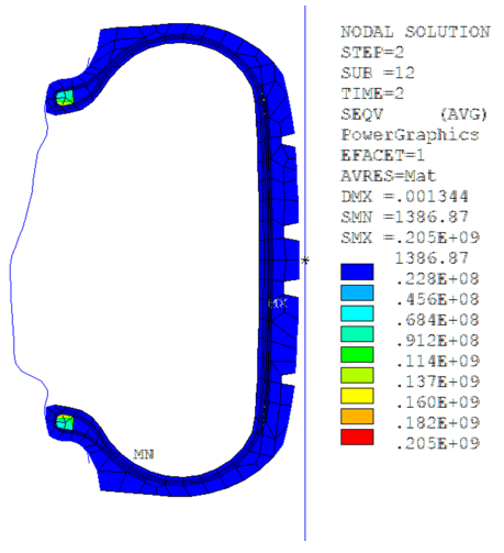
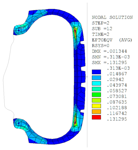
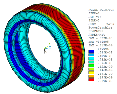
Following are the equivalent stress and equivalent total strain plots from the inflation analysis on the 2D axisymmetric tire model:

Figure 57.24: Equivalent Stress

Figure 57.25: Total Equivalent Strain

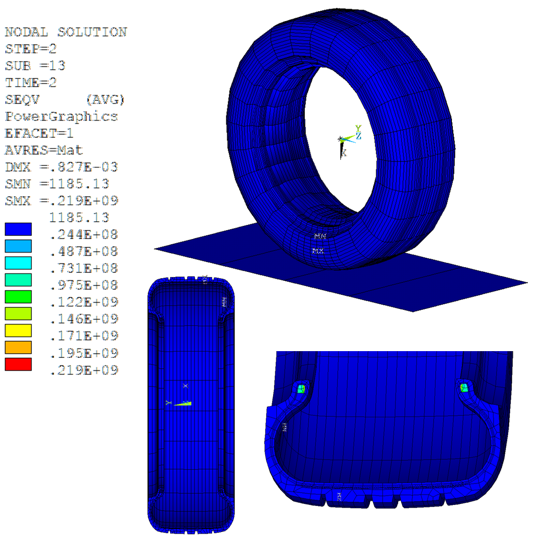
With solid-shape display enabled (/ESHAPE,1), the following plot shows the equivalent stress on the 2D reinforcing elements (in the belt and body-ply regions) after the rim-mounting and inflation analyses on the 2D axisymmetric model:

Figure 57.26: Equivalent Stress on the 2D Reinforcing Elements (3D Model)

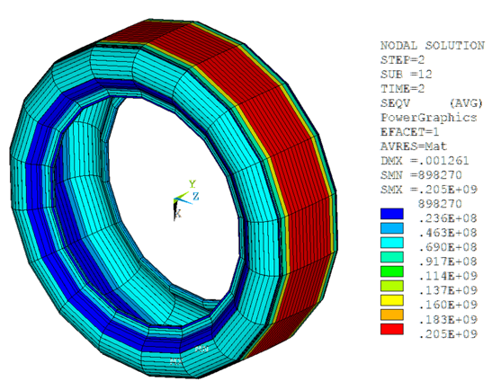
As expected, the maximum equivalent stress is observed in the belts region.

Following is the equivalent stress plot on the reinforcing elements of the extruded 3D tire model (EEXTRUDE) after the mapping operation (MAP2DTO3D):

Figure 57.27: Equivalent Stress on 3D Reinforcing Elements After Mapping

Following are the equivalent stress and total mechanical equivalent strain plots on the extruded 3D tire model after mapping:

Figure 57.28: Equivalent Stress Plot After Mapping

Figure 57.29: Total Mechanical Equivalent Strain Plot After Mapping

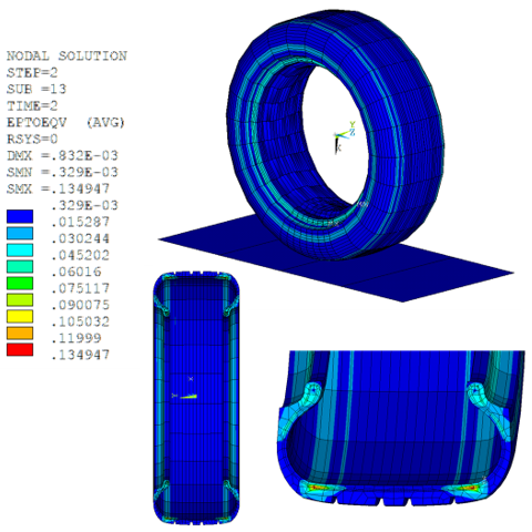
As expected, the results closely match those of the corresponding 2D model.

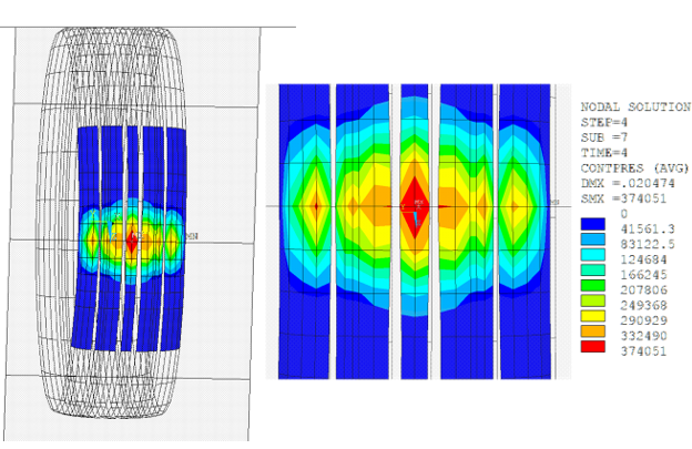
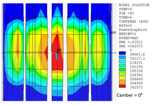
Following is the contact-pressure distribution for the road-tire contact pair after the footprint analysis:

Figure 57.30: Contact-Pressure Distribution on the Road-Tire Contact Pair (Camber = 0°)

Figure 57.31: Contact-Pressure Distributions at Various Camber Angles

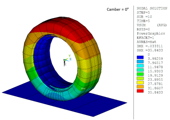
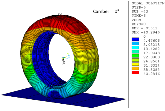
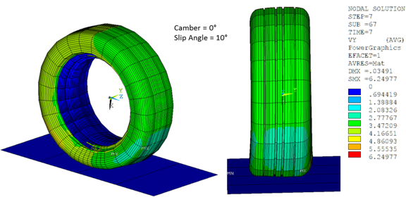
With the tire in a braking condition, following is the velocity vector sum plot (VSUM) after the first steady-state rolling analysis:

Figure 57.32: Steady-State Rolling (ω1= 50 rad/s, Vz = 20 m/s, Camber = 0°)

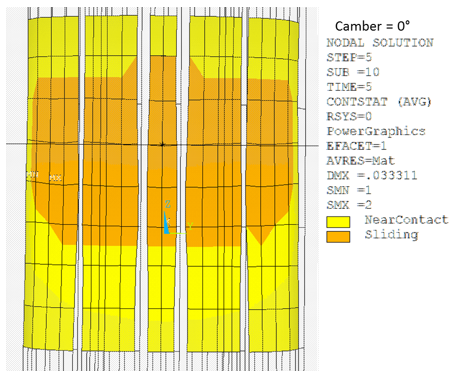
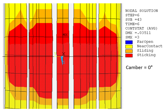
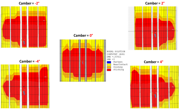
For the road-tire contact pair, most of the contact patch is in a sliding state:

Figure 57.33: Road-Tire Contact-Pair Status at Steady-State Rolling (ω1= 50 rad/s, Vz = 20 m/s)

In the free-rolling analysis with 0° camber, the variation of longitudinal reaction force (Fz) at the pilot node of the tire-rim contact pair is as follows:

Figure 57.34: Variation of Longitudinal Reaction Force (Fz)

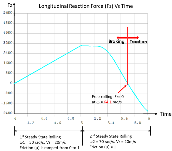
Two steady-state rolling analyses follow the footprint analysis:

Fz changes from positive to negative values during the second steady-state rolling analysis, meaning that the tire’s rolling state is transitioning from a braking state to traction state. Free-rolling occurs when Fz = 0.

Figure 57.35: Free-Rolling State Velocity Vector Sum (ω1= 64.1 rad/s, Vz = 20 m/s, Camber = 0°)

Following are results plots for the road-tire contact pair at the free-rolling state:

Figure 57.36: Free-Rolling State Contact-Pressure Distribution (Camber = 0°)

Figure 57.37: Free-Rolling State Contact Status (Camber = 0°)

Figure 57.38: Free-Rolling Contact-Pressure Distributions at Various Camber Angles

Figure 57.39: Free-Rolling Contact Statuses at Various Camber Angles

Following the cornering analysis, the velocity plot in the lateral direction (Vy) is:

Figure 57.40: Velocity in the Lateral Direction (Vy) Following Cornering Analysis (Slip = 10°, Camber = 0°)

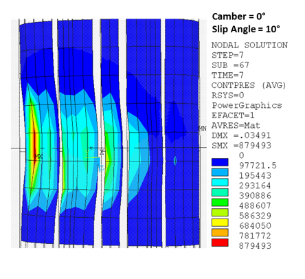
Following is the results plot for the road-tire contact pair after the cornering analysis:

Figure 57.41: Cornering Contact-Pressure Distribution (Slip = 10°, Camber = 0°)

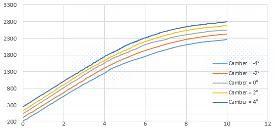
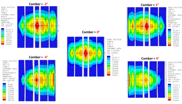
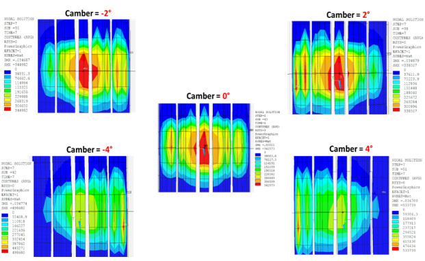
At various camber angles, the cornering-force (Fy) variation with respect to the slip angle shows that the corning force is proportional to the slip angle at low slip angles:

Figure 57.42: Cornering Force (Fy) vs. Slip Angle for Various Camber Angles