The natural frequencies of the 2D axisymmetric model without rotation are evaluated and compared with the results of 3D solid model in the following table.

The natural frequencies of the 2D axisymmetric model in rotation (50,000 rpm) also show good agreement with the 3D solid model results, as shown in the following table.

The /POST1 results of the Campbell diagram analysis are shown in the figure that follows.

Figure 14.15: Campbell Diagram

2D Axisymmetric Model

3D Solid Model

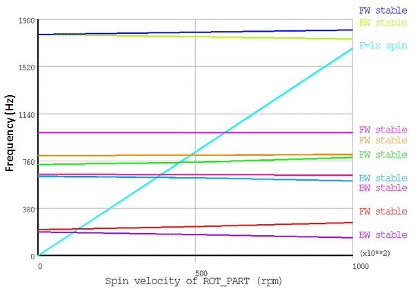
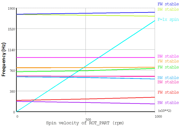
With the help of the Campbell diagram analysis, one can identify the forward (FW) and backward (BW) whirls, as well as possible unstable frequencies (though none are present in this example). In the table below, the whirls and natural frequencies of the 2D axisymmetric model at maximum rotational speed (100,000rpm) are compared with the 3D solid model results.

The Campbell diagram analysis helps to determine the critical speeds of the rotating structure (PRCAMP ). Critical speeds are compared in the table below. For a synchronous excitation, the critical speeds correspond to the intersection points between the frequency curves and the 1.0 slope line. The critical speeds of the 2D axisymmetric and 3D solid models show strong agreement.

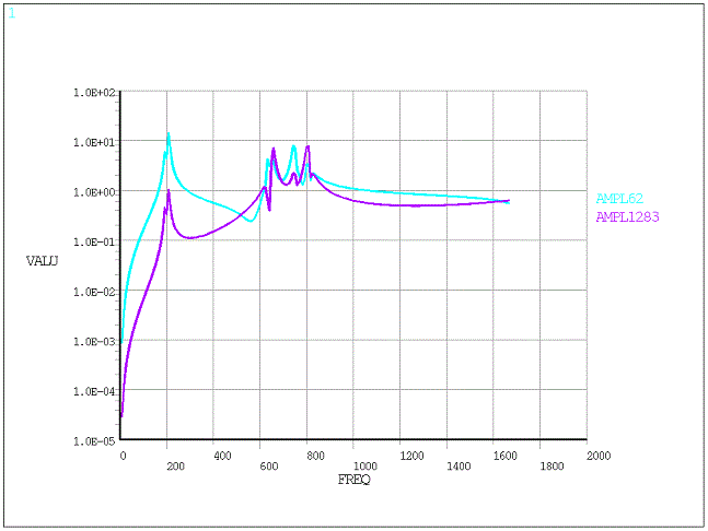
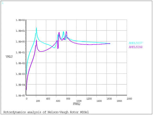
The results of the unbalance response analysis post processed in /POST26 are shown in the following figure. The logarithmic plots show the variation of the displacement amplitudes of two selected nodes with respect to the frequency of excitation. The first node is located near the rigid disk, and it corresponds to the light blue curve. The second node is located near the bearing location, and it corresponds to the purple curve.

The critical frequencies appear where the amplitudes are largest, and correspond to the critical speeds.

Figure 14.16: Unbalance Response

2D Axisymmetric Model

3D Solid Model

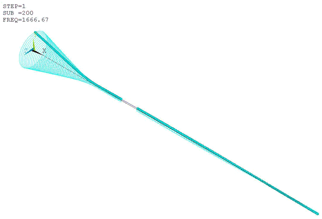
The orbits after a full harmonic analysis can be plotted in POST1 (PLORB) as shown in the figure below. For the solid element and the axisymmetric element model, it is necessary to add massless line elements using BEAM188 on the rotational velocity axis to plot these orbits. The orbits of the 2D axisymmetric model at a frequency of 1666.67 Hz are shown in the figure below. The rotor line is in dark blue, while the orbits are in light blue.

The following input fragment shows the steps to produce an orbits plot at a given frequency:

/POST1
esel,r,ename,, 188  ! Select BEAM188 elements to produce orbits
set,1, 200          ! Visualize orbits at frequency 1666.67 Hz 
/view,,1,1,1
plorb               ! Displays the orbital motion of a rotating structure

Figure 14.17: Orbits Plot of 2D Axisymmetric Model

 

14.7.1. Performance Benefits of the 2D Axisymmetric Model

The memory and CPU usage of the 2D model is shown in the following table.

	2D Axisymmetric Model
	Elements #	Nodes #	No. of Equations	Memory required for in-core (MB)	CPU Time (Sec)
Campbell Diagram Analysis	2208	6751	20225	53.283	17.30
Unbalance Response Analysis				118.325	1347.53

The memory and CPU usage of the 3D model is shown in the following table.

	3D Solid Model
	Elements #	Nodes #	No. of Equations	Memory required for in-core (MB)	CPU Time (Sec)
Campbell Diagram Analysis	9239	15123	45341	186.141	45.56
Unbalance Response Analysis				605.464	4645.95

The CPU times for the unbalance response analysis are represented in the following bar graph.

Figure 14.18: CPU Time of 2D Axisymmetric and 3D Solid Models (Unbalance Response Analysis)