


The meshed 2-D plain strain model that represents the cylinder on the flat slab is shown in the following figure.
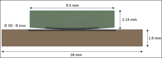
The global element size is set to 0.100 mm. The mesh is refined in the central zone
(LEVEL = 3) for better stress-strain resolution.
The geometry is meshed with 2-D plain strain PLANE182 elements (KEYOPT(3) = 2). Frictional contact (µ = 0.80) is modeled between the half cylinder and the flat slab by overlaying their surfaces with contact elements (CONTA172) and target elements (TARGE169). The model uses symmetric contact to simulate wear on the cylinder and flat slab. Contact and target elements are defined on both surfaces as wear can only be modeled on surfaces with contact elements.
The (CONTA172) elements have the following settings:
KEYOPT(2) = 0 - Augmented Lagrange formulation.
KEYOPT(10) = 0 - Contact stiffness updates at each iteration.
KEYOPT(4) = 3 - Location of the contact detection point: on nodal point - normal from contact surface (standard projection-based method).
Wear is simulated by defining a wear model (TB,WEAR), and assigning it to the contact elements using the generalized form of the Archard wear model:
TB,WEAR,CID,,,ARCDContact elements are defined on the surfaces undergoing wear, and CID is the material ID associated with the contact elements. Wear on the half cylinder is defined as:
kwear = 2.75e-8
TB,WEAR,3,,,ARCD        ! Mat #3 = material for wear contact element on the cylinder
TBFIELD,TIME,0          ! Time at the beginning of load step 1
TBDATA,1,0,1,1,1,0      ! C1 = 0 results in no wear for load step 1
TBFIELD,TIME,1          ! Time at the end of load step 1
TBDATA,1,0,1,1,1,1      ! C1 = 0 results in no wear for load step 1
TBFIELD,TIME,1.01       ! Time at the beginning of load step 2
TBDATA,1,kwear,1,1,1,0  ! Value of wear coefficient resulting in initiation of wear
TBFIELD,TIME,4          ! Time at the end of load step 2
TBDATA,1,kwear,1,1,1,0  ! Wear coefficient kept constant during load step 2
Wear on the flat slab is defined as:
kwear = 2.75e-8
TB,WEAR,4,,,ARCD        ! Mat #4 = material for wear of contact element on flat
TBFIELD,TIME, 0         ! Time at the beginning of load step 1
TBDATA,1,0,1,1,1        ! C1 = 0 results in no wear for load step 1
TBFIELD,TIME,1          ! Time at the end of load step 1
TBDATA,1,0,1,1,1        ! C1 = 0 results in no wear for load step 1
TBFIELD,TIME,1.01       ! Time at the beginning of load step 2
TBDATA,1,kwear,1,1,1    ! Value of wear coefficient resulting in start of wear
TBFIELD,TIME,4          ! Time at the end of load step 2
TBDATA,1,kwear,1,1,1    ! Wear coefficient kept constant during load step 2
Specifying Automatic Wear Scaling
To speed-up the wear process, two adaptive wear scaling methods are used with following scaling parameters:
TB,WEAR,CID,,,AUTS     ! Adaptive wear scaling for Mat #3
TBDATA,1,0.1,1000      ! Wear scaling parameters
TB,WEAR,TID,,,AUTS     ! Adaptive wear scaling for Mat #4
TBDATA,1,0.1,1000      ! Wear scaling parameters
In automatic wear scaling (AUTS), wear is scaled and the geometry is updated at each sub-step using the wear scale factor calculated at the previous sub-step. For dynamic wear rate problems, wear scale factors may vary within a simulation cycle. Using a sufficiently small value for the maximum allowable wear scale, a constant wear scale factor within a simulation cycle could be obtained.
For both scaling methods, the first parameter (0.10) represents the safety factor that controls wear depth in terms of the penetration locally. The second parameter (1000) specifies the maximum allowable wear scale factor (Automatic Scaling of Wear Increment) for a contact interface. The maximum allowable wear scale factor is set to the ratio of estimated life cycles to simulation cycles for a smaller number of simulation cycles. Too large a value for the maximum allowable wear scale factor may lead to inaccuracy or even numerical instability. These scaling factors should not affect the estimated fretting fatigue life.
Modeling wear involves repositioning contact surface nodes to simulate the material removal process. As a result, the solid elements underlying the contact elements can quickly deteriorate. Nonlinear mesh adaptivity is used to resolve mesh distortion issues. A component is created named “conwearel”, and the following command triggers mesh adaptivity:
allsel,all
esel,s,ename,,169,172,3
cm,conwearel,elem
nlad,conwearel,add,contact,wear,0.50    !morph after 50% is lost in wear
nlad,conwearel,on,all,all,1,,4
nlad,conwearel,list,all,all
In this case, adaptivity occurs whenever wear at any contact point exceeds 50% of the average height of the solid element underlying the contact element. Each time the criterion is reached, the analysis is stopped, the mesh quality is improved by morphing the mesh, history-dependent variables and boundary conditions are mapped, and the analysis is restarted with an improved mesh. This is an automatic process.