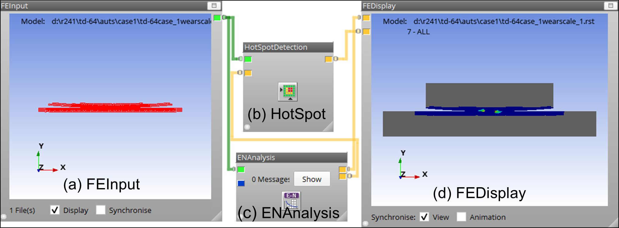
You can use nCode DesignLife within Ansys Mechanical or the standalone version of nCode DesignLife (if an FE result file is available) to postprocess fatigue modeling results. The nCode fatigue workflow is built into Ansys Mechanical with an integrated workflow. Standalone nCode DesignLife is used for this example problem to calcluate fretting fatigue life with wear. Download the most recent available nCode package at https://download.ansys.com/Current%20Release under Add-on Packages. The GUI is similar to the integrated version of nCode in the Mechanical Application. Set up the workflow as shown in the following figure using drag and drop options of the nCode menu. Details of the setup are as follows:
| (a) FE Input - critical element component (where failure is expected) is performed in MAPDL for faster fatigue analysis. |
| (b) HotSpot - selects a specified number of critical points in the selected critical component. |
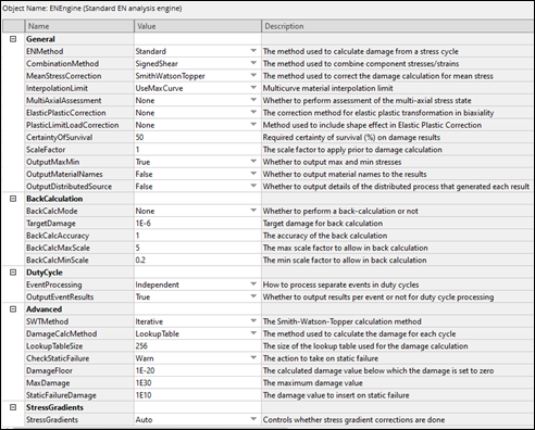
| (c) ENAnalysis - the main fatigue calculation engine, where material, load, and analysis specification are made. |
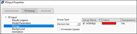
| (d)FEDisplay - shows the calculated life/damage. |
Figure 64.4: Standalone nCode DesignLife Workflow: (a) FE Input, (b) HotSpot, (c) ENAnalysis, and (d) FEDisplay
For the fretting fatigue analysis, select the four main building blocks and make connections between them as shown in the figure. Right mouse click ENAnalysis and specify the following fretting fatigue damage parameters under advance edit. Snippets of some important parameters are shown below.
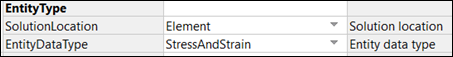
(a) FE Results
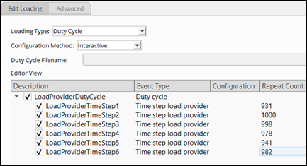
(b) Load Provider
Stress and strain evolve over time as the geometry at the interface changes with wear. Use the time-step load provider to account for a varying load history. To calculate fretting damage with wear, the FE model is solved for a few simulation cycles with scaled wear. For example, the first simulation cycle starts at 1.0000 and ends 1.5000 sec. The simulation time is scaled with the same scaling factor as the wear process to estimate the physical time. The physical time for the first cycle starts at 1.0000 s and ends at 466.353 for d = 0.000 mm Fy = -208.4 N/mm. Repeat counts are calculated by comparing the physical and simulation cycle period, as shown in Table 64.1: Calculating repeat counts for each simulation cycle Fy = - 208.4N/mm, auto wear scaling (auts). Each simulation cycle is combined into aduty cycles that serves as a time step load provider. The summary of the load setting is given below for d = 0.000 mm with auto scaling (AUTS).
(c) Material map
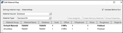
For the fast fatigue calculation, HTSPTELE is a component of elements where failure is expected. the fatigue calculation time is reduced by performing the fatigue analysis on only the selected group of elements.
(d) Analysis runs

(e) Failure criterion
The signed-Shear combination method with Smith-Watson-Topper (SWT) mean stress correction was found to predict fretting fatigue life more accurately for Ti6Al4V material.
(f) Results
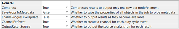
To obtain the accumulated damage in each simulation cycle, set channel per event to “True”.