This example shows the nonlinear harmonic analysis of two jointed beams with a frictional contact interface using Harmonic Balance Method (HBM). Specifically, it demonstrates the following key points:
The example problem is presented in the following sections:
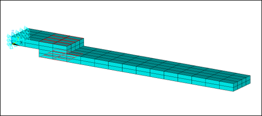
Two solid beams of respective sizes 40 x 20 x 5 mm and 140 x 20 x 5 mm are meshed with SOLID185 elements and linked by a frictional contact interface of 20 mm length. The left end of the top beam is clamped, and a constant surface pressure of magnitude 1 N/mm2 is applied on each side of the contact area to maintain contact between the two beams.
All node-to-node contact elements have a normal and tangential stiffness of 103 N/m and a friction coefficient of 0.3.
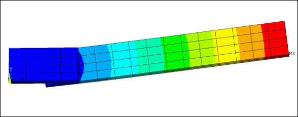
The first out-of-plane mode of the jointed beams (f2 = 318.7 Hz), which generates high friction in the joint interface is under study in the nonlinear harmonic analysis. It is activated by applying a transverse surface pressure of different magnitude levels at the end of the lower beam. To compute the response, the frequency range for the HBM analysis is [310, 325] Hz and the number of harmonics NH = 3.
Model reduction
Before running the HBM analysis, the linear part of the model is condensed using Component Mode Synthesis (CMS) to reduce the total number of equations and consequently the computational time. The 15 nodes on each substructure used to define contact and one observation node at the end of the lower beam are selected as master nodes. Loads are defined using superelement load vectors to apply pressure, avoiding extra master nodes for loading. Six modes are used to generate each superelement so that the total number of HBM equations is 735.
Preload
To improve convergence at the first frequency point, a preliminary static analysis is run considering only the constant pressure load. Then, the static solution is read from the results (Jobname.rst) file and used as an initial guess for the HBM solution (HBMOPT,UINIT). The procedure to define the HBM initial guess is as follows:
Combine the static Jobname.full files if using distributed-memory parallel (DMP) processing.
Read the static solution vector to be used as the 0th harmonic (
) of the initial guess (
) from the Jobname.rst file.
Create the multiharmonic solution vector (
in Equation 1–7 - Equation 1–9, referred to here as
for clarity) using the *DIM command. The size of
is related to
and the number of harmonics NH as follows:
size(
) = size(
)*(2*NH + 1).
Fill the
vector with
values.
is defined as
= [
;
;
;
;
; … ;
]
where
the subscripts
and
denote real and complex values
and the integer superscripts denote the time-domain harmonic index h (see Equation 1–9).
Read the BACK nodal mapping vector from the Jobname.rst file and export it to an APDL array named "UserBack".
Specify the initial guess for the HBM solution using
and UserBack as inputs by issuing HBMOPT,UINIT,APDL,umh,INT,UserBack.
The HBM initial guess can be retrieved from different preliminary analyses. See below for more details about the procedure.
To restart from a linear harmonic analysis, use
the linear solution as an initial guess to help the solver converge towards the
first solution. Follow the procedure described above except for steps two and four
to fill the multiharmonic solution vector :
| 2. Read the linear harmonic solution vector (real |
| 4. Fill the |
To resume a prior HBM analysis that stopped due to convergence failure or a stopping criterion, restart the analysis at the last point computed. Changing some parameters (number of harmonics NH, number of time points per period NT, etc. via HBMOPT) without recomputing the previous substeps reduces the workflow and computation time. Follow the procedure described above except for steps two and four to fill the multiharmonic solution vector umh (see Example 8.1: Command Input for Filling umh from a Previous HBM Analysis):
| 2. For each harmonic of the initial run, read the solution vector (real
|
| 4. Fill the |
Example 8.1: Command Input for Filling umh from a Previous HBM Analysis
! number of harmonics
NH = 3

*get,rstName,active,,jobnam
*VEC,u0,D,IMPORT,RST,%rstName%.rst,1,,NSL
uDim = u0_Dim ! size of the single harmonic solution vector

! size of the multiharmonic solution vector
umhDim = uDim*(1+2*NH)
*DIM,umh,ARRAY,umhDim

! fill vector with harmonic 0 solution
*DO,i,1,uDim
   umh(i) = u0(i)
*ENDDO

! fill vector with other harmonic solutions (complex)
iloc = uDim
*DO,ih,1,NH
   *VEC,uh,Z,IMPORT,RST,%rstName%_%ih%hi0.rst,iRestart,,NSL
   *DO,i,1,uDim
      iloc = iloc + 1
      umh(iloc) = uh(i,1)
   *ENDDO
   *DO,i,1,uDim
      iloc = iloc + 1
      umh(iloc) = uh(i,2)
   *ENDDO
*ENDDO
Scaling the solution vector
To improve convergence behavior in the Newton-Raphson continuation procedure, the use of HBMOPT,SCAL to linearly scale each component of the solution vector by providing a vector of scaling factors is demonstrated here. (For scaling equations and tips on scaling the solution vector, see Equation Solution and Scaling the Solution Vector.)
Scaling the solution to improve convergence depends on the specifics of each model. Although there is no universal rule for determining scaling factors, the approach and equations used in this problem are often applicable. Since scaling does not affect solution accuracy, you can use typical or approximate values (as exact values may be unknown a priori) or other strategies to determine scaling parameters suitable for your application.
For this problem, the scaling vector is defined as an APDL array named "uscal" filled with a constant scaling factor for the displacement, scal_disp. The number of physical equations, Neq_typ, and the largest predicted displacement, Umax_typ, are used to calculate the displacement scaling factor by scal_disp = Neq_typ*Umax_typ. A value of scal_freq =300*2*p, close to the frequency range of interest (in rad/s) is used to scale the solution degree of freedom which corresponds to the forcing frequency. Finally, the scaling is applied by issuing HBMOPT,SCAL,1,uscal,scal_freq,SOLU. Note that for this example, a constant scaling value could be used (HBMOPT,SCAL,VALU,scal_disp,scal_freq), and a vector is created only for demonstration purposes.
To download the .dat file used for this example problem, click the link below.
The contents of this file are listed below. The command listing shows in detail how to specify and run the HBM analysis. You can use it as a template and modify it to create a custom HBM analysis.
/batch,list
/title, Two jointed beams with frictional contact interface

! beam 1
Lb1 =  40                           ! length
wb1 =  20                           ! width
tb1 =   5                           ! thickness

! beam 2
Lb2 = 140                           ! length
wb2 =  20                           ! width
tb2 =   5                           ! thickness

! material
E   = 116e3                         ! Young's modulus
nu  = 0.32                          ! Poisson's ratio
rho = 4506e-12                      ! density

alpd = 2e-6                         ! alpha damping
betd = 1e-5                         ! beta damping

! contact
Lc = 20                             ! surface length
wc = 20                             ! surface width
Kn = 1e3                            ! normal     stiffness
Kt = 1e3                            ! tangential stiffness
mu = 0.3                            ! friction coefficient

! load
FN0 = 1.0                           ! static   pressure
FT1 = 5.0e-4                        ! harmonic tangential force
                                    ! 1.0e-4, 5.0e-4, 1.0e-3 or 2.0e-3 to reproduce figure 3 results

! mesh
esiz_x = Lb1/4                      ! element size in x-direction
esiz_y = wb1/4                      ! element size in y-direction
esiz_z = tb1/2                      ! element size in z-direction

! CMS
Nmode = 6

! HBM
Fmin  = 310
Fmax  = 325

NH    = 3                           ! number of harmonics

ds    = 0.5                         ! initial step size
dsmin = ds/50                       ! minimum step size
dsmax = ds*5                        ! maximum step size

neq_hbm   = (31*3+2*Nmode)*(2*NH+1) ! number of HBM equations:
                                    !      113 equations = 31 nodes X 3 dofs + 20 CMS modes

pi        = acos(-1)

! typical values of the problem
Neq_typ   = 90                      ! typical number of physical equations
Umax_typ  = 0.10                    ! typical value of maximum displacement (mm)
Fpeak_typ = 300                     ! peak frequency (Hz)

! scaling values
scal_disp = Umax_typ*Neq_typ        ! scaling for displacement DOFs
scal_freq = 2*pi*Fpeak_typ          ! scaling for frequency    DOF

/prep7

! material
mp,ex  ,1,E
mp,prxy,1,nu
mp,dens,1,rho
mp,alpd,1,alpd
mp,betd,1,betd

mp,mu,2,mu

! geometry
block, 0,Lb1,             0,wb1, 0,tb1  ! beam 1
block, Lb1-Lc,Lb1+Lb2-Lc, 0,wb2, -tb2,0 ! beam 2

! element types
et,1,185

! mesh
vsel,s,volu,,1,,,1
lsel,r,loc,x,Lb1/2
lesize,all,esiz_x
allsel

vsel,s,volu,,2,,,1
lsel,r,loc,x,Lb1-Lc+Lb2/2
lesize,all,esiz_x
allsel

lsel,s,loc,y,wb1/2
lesize,all,esiz_y
allsel

lsel,s,loc,z, tb1/2
lsel,a,loc,z,-tb2/2
lesize,all,esiz_z
allsel

type,1
real,1
mat ,1
vmesh,all

vsel,s,volu,,1,,,1
cm,beam1_node,node
cm,beam1_elem,elem
allsel

vsel,s,volu,,2,,,1
cm,beam2_node,node
cm,beam2_elem,elem
allsel

finish

save,full,db
parsav,all,full,parm

/com
/com ______________ GENERATION PASS - BEAM 1 _____________
/com
/filname,beam1

/solu
antype,substr
seopt,beam1,3,,,NONE        ! generate stiffness, damping, and mass matrix
                            !          (NONE = no files kept for expansion)
cmsopt,fixed,Nmode

! boundary conditions
nsel,s,loc,x,0
d,all,all
allsel

! loading
nsel,s,loc,x,Lb1-Lc,Lb1
nsel,r,loc,z,tb1
sf,all,pres,1
allsel

! master dofs
cmsel,s,beam1_node
nsel,r,loc,z,0
nsel,r,loc,x,Lb1-Lc,Lb1
cm,contact_beam1,node
allsel

cmsel,s,contact_beam1
m,all,all
allsel

cmsel,s,beam1_node      ! select only nodes and elements for beam 1
cmsel,s,beam1_elem
solve
finish

save

/com
/com ______________ GENERATION PASS - BEAM 2 _____________
/com
/filname,beam2

/solu
antype,substr
seopt,beam2,3,,,NONE   ! generate stiffness, damping, and mass matrix
                       !          (NONE = no files kept for expansion)
cmsopt,fixed,nmode

! master dofs
cmsel,s,beam2_node
nsel,r,loc,z,0
nsel,r,loc,x,Lb1-Lc,Lb1
cm,contact_beam2,node
allsel

nsel,s,loc,x,Lb1-Lc+Lb2
nsel,r,loc,y,wb2/2
nsel,r,loc,z,0
cm,load_beam2,node
allsel

cmsel,s,contact_beam2
cmsel,a,load_beam2
m,all,all
allsel

/com >>>>>> LOAD VECTOR 1
nsel,s,loc,x,Lb1-Lc,Lb1
nsel,r,loc,z,-tb2
sf,all,pres,1
allsel

cmsel,s,beam2_node     ! select only nodes and elements for beam 2
cmsel,s,beam2_elem
solve

/com >>>>>> LOAD VECTOR 2
sfdele,all,all
nsel,s,loc,x,Lb1+Lb2-Lc
sfco,2,,0,1,0
sf,all,pres,1
allsel

cmsel,s,beam2_node     ! select only nodes and elements for beam 2
cmsel,s,beam2_elem
solve

finish

save

/com
/com ______________ USE PASS _____________
/com
/clear,nostart
/filname,hbm

parres,,full,parm

/prep7

! load SE
et,10,50
type,10
se,beam1
se,beam2

! contact
et,2,178
keyopt,2,2 ,1        ! pure penalty method
keyopt,2,5 ,3        ! contact normal along z-direction
r,2,-Kn,,,-Kt

mp,mu,2,mu

type,2
real,2
mat ,2
nsel,s,loc,z,0
nsel,r,loc,x,Lb1-Lc,Lb1
eintf,,,HIGH
allsel

finish

/solu
antype,static

rescontrol,define,last,last
nropt,unsym

! boundary conditions
nsel,s,loc,x,0
d,all,all
allsel

! loading - constant pressure
sfe,1,1,SELV,0,FN0 ! SE 1 - LV 1
sfe,2,1,SELV,0,FN0 ! SE 2 - LV 1

solve
finish
save

/clear,nostart
/filname,hbm

resume,hbm,db

/com
/com ---- READ STATIC RESULTS AND WRITE CORRESPONDING HBM INITIAL SOLUTION VECTOR
/com

! read harmonic 0 solution (real)
*get,jobn,active,,jobnam
*VEC,u0,D,IMPORT,RST,%jobn%.rst,1,,NSL
uDim   = u0_Dim                     ! size of the single harmonic solution vector
umhDim = uDim*(1+2*NH)              ! size of the multiharmonic solution vector

! fill multiharmonic vector with harmonic 0 solution
*DIM,umh,ARRAY,umhDim
*DO,i,1,uDim
   umh(i) = u0(i)
*ENDDO

! read the mapping
*xpl,open,%jobn%.rst
*xpl,read,nod,BackVecI
*xpl,close
*vec,BackVecD,D,copy,BackVecI
*export,BackVecD,apdl,UserBack

/solu
antype,harmic

hropt,hbm,NH                        ! hbm solve and number of harmonics
harfrq,Fmin,Fmax

hbmopt,contset,,ds,dsmin,dsmax
hbmopt,uinit,APDL,umh,INT,UserBack
hbmopt,contterm,100,50
hbmopt,nr,10

kbc,1

! boundary conditions
nsel,s,loc,x,0
d,all,all
allsel

! loading - constant pressure - harmonic 0
*dim,FNtab,TABLE,NH+1,1,,NHINDEX,FREQ
*vfill,FNtab(1,0),RAMP,0,1
FNtab(0,1) = 100
FNtab(1,1) = FN0
sfe,1,1,SELV,0,%FNtab%              ! SE 1 - LV 1
sfe,2,1,SELV,0,%FNtab%              ! SE 2 - LV 1

! loading - tangential pressure - harmonic 1
sfe,2,2,SELV,0,FT1                  ! SE 2 - LV 2

! scaling
*dim,uscal,array,neq_hbm
*vfill,uscal(1),RAMP,scal_disp,0

hbmopt,scal,1,uscal,scal_freq,SOLU

solve
finish

/post26

nsel,s,loc,x,Lb1-Lc+Lb2
nsel,r,loc,y,wb2/2
nsel,r,loc,z,0
nd_load = ndnext(0)
allsel

HBM_EXPA,'hbm',nd_load,'u','y',NH,'minmax'

*vfact,1/(FT1*wb2*tb2)
*vfun,_hbm_ampl(1),COPY,_hbm_ampl(1)

/gmarker,,4
/xrange,310,325
/yrange,0,3
/axlab,X,Frequency (Hz)
/axlab,Y,Amplitude (mm/N)
/plopt,info,0
/title,Ft = %FT1% N
/show,png,rev
   *vplot,_hbm_freq(1),_hbm_ampl(1)
/show,close

/nopr
/out,results_FT%FT1%,txt
*vwrite,_hbm_freq(1),_hbm_ampl(1)
(F10.5,' , ',E12.6)
/out,scratch

finish
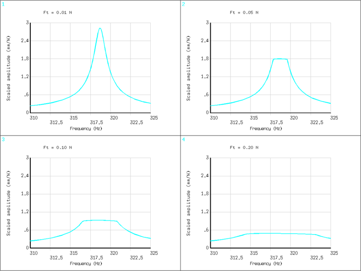
The amplitude of UY displacement at the tip of the lower beam is computed using the HBM_EXPA macro. The amplitude of the response scaled by the excitation amplitude is shown in the figure below for different levels of excitations.
It shows that friction dissipates energy because of the contact stick-slip phenomenon. When increasing the excitation amplitude from 0.01 N to 0.20 N, the scaled amplitude of the response decreases. This corresponds to an increase of frictional damping due to the contact elements spending more time in the sliding state.
Information about the contact status is provided in the jobname1.out file for each iteration. For example, for Ft = 0.10 N and close to the natural frequency, the summary shows that sliding occurs on average 12.5% of time for 2 of the 15 contact elements:
******** SUMMARY OF CONTACT ELEMENTS BEHAVIOR DURING LAST PERIOD ********
NO. OF ELEMENTS STICKING AT LEAST ONCE =  15  | AVERAGE % OF TIME =  98.3%
NO. OF ELEMENTS SLIDING AT LEAST ONCE  =   2  | AVERAGE % OF TIME =  12.5%
For Ft = 0.20 N and around the same frequency, there are still only 2 elements sliding but they spend a greater time sliding, on average of 20% of the time:
******** SUMMARY OF CONTACT ELEMENTS BEHAVIOR DURING LAST PERIOD ********
NO. OF ELEMENTS STICKING AT LEAST ONCE =  15  | AVERAGE % OF TIME =  97.3%
NO. OF ELEMENTS SLIDING AT LEAST ONCE  =   2  | AVERAGE % OF TIME =  20.3%


