


A Microstructure Simulation produces one summary result page (the parent simulation) showing the set of permutations (child simulations) included within it. Selecting any of the permutations brings up a new page of individual permutation results. These results include:
The microstructure in XY, YZ, and XZ planes available in both .avz format that can be viewed and exported, and as .vtk files that can be exported. Use these data to view grain orientation, grain boundaries, and grain number.
Grain size statistics available in both summary bar graph form that can be viewed and .csv files that can be exported.
Viewing Grain Orientation
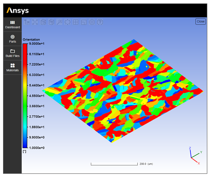
The three primary result items in a Microstructure Simulation are grain orientation angle, grain boundaries, and grain number. Grain orientation represents grain growth direction with respect to the horizontal axis of a 2D plane based on a moving heat source. Note that it does not represent crystal orientation that is typically seen in an EBSD map. Grain orientation angles from an individual permutation are shown in the following figure when viewed in the application (AVZ viewer). A unique grain number is assigned to one continuous grain. A unique color is assigned for each orientation.
To view all three planes at once, use Ansys EnSight, a tool for high performance graphics post-processing. (Alternatively, you can use an open-source visualization application such as Paraview.) Within EnSight, visualize the microstructure data by doing the following:
Choose File > Open to open any one of the three plane .vtk files. This will provide data to the default “Case 1”, which can be renamed by right-clicking and choosing “Rename case…”.
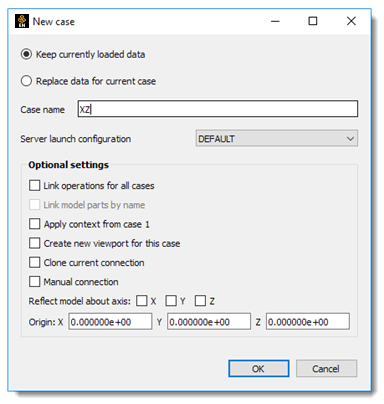
Repeat File > Open for the next two planes, selecting “Keep currently loaded data” when the “New case” dialog box appears. Change case name, if desired.
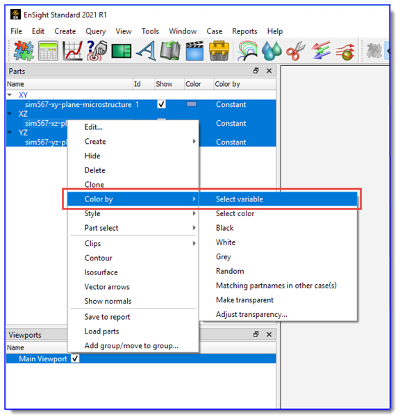
Click and drag or use Ctrl + click to select all three data cases in the data panel.
Right-click and select Color by > Select variable.
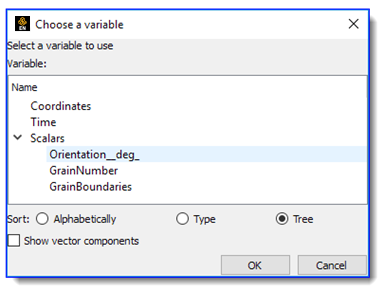
Under Scalars, choose the desired variable (orientation, grain number, or grain boundaries). Click OK.
Changing the color palette may provide more contrast among individual grains, depending on your selected variable. Right-click the legend and then select Palette > Edit palette.
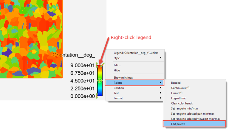
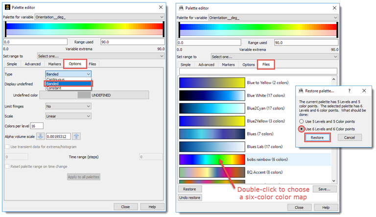
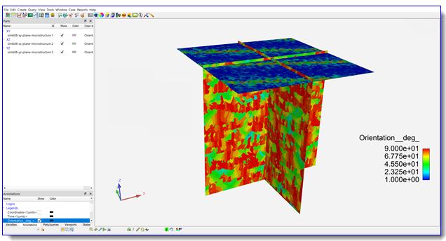
In the Palette editor, under the Options tab, choose Banded for the type of color distribution. Preset color maps can be chosen under the “Files” tab by double-clicking on the desired color map. To view grain orientation, we recommend using a six-color color map. Click Restore to activate your chosen color map.
Use the pan, rotate and zoom controls to achieve the desired view. Right-click anywhere in the viewport and under View, select any of the view directions to return to a specific plane.
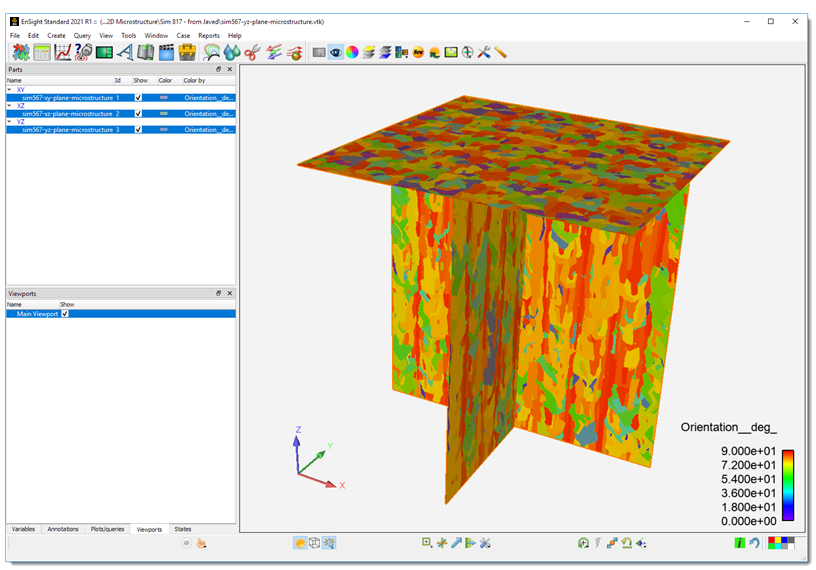
If the sensor height is not evenly divisible by the layer thickness, the vertical planes (XZ and YZ) may extend through the XY plane as shown in the next figure.
Viewing Grain Boundaries
The purpose of the grain boundaries map is to see only the boundaries of the grains, similar to grain scale images seen in optical microscopy. Internally, this two-color effect is achieved by setting a grain boundary flag to 1 and the interior to 0.
As an example, using the EnSight instructions in the previous section:
Choose File > Open to open the XZ plane .vtk file. Rename Case 1 to XZ plane.
Select the XZ plane, right-click and select Color by > Select variable.
Under Scalars, choose grain boundaries. Click OK.
Right-click the legend and then select Palette > Edit palette.
For best viewing of the grain boundaries, we recommend using the “X Ray (2 colors)” option in the Palette editor. In the Palette editor, under the “Files” tab, double-click the “X Ray (2 colors)” color map.
Right-click anywhere in the viewport and under View, select the -Y view to see the XZ plane.
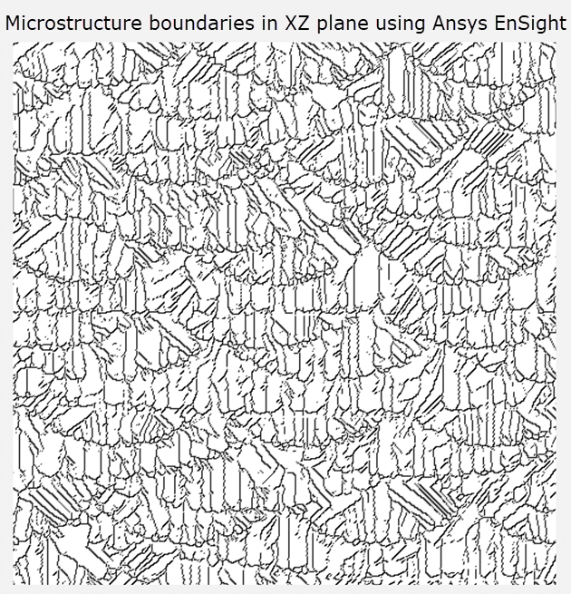
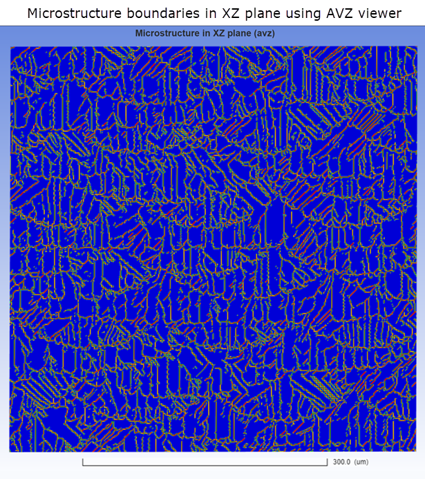
The same grain boundaries data are shown next in the AVZ viewer.
Viewing Grain Size Statistics
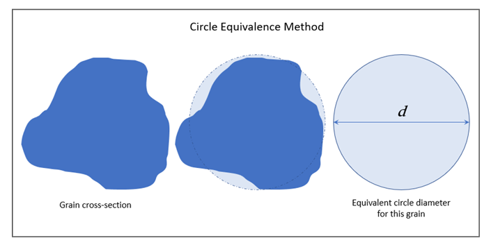
For each grain, the area and the area fraction of the total area are calculated. To do this, the diameter of an equivalent circle for each grain is calculated using the Circle Equivalence Method, as shown in the following figure.
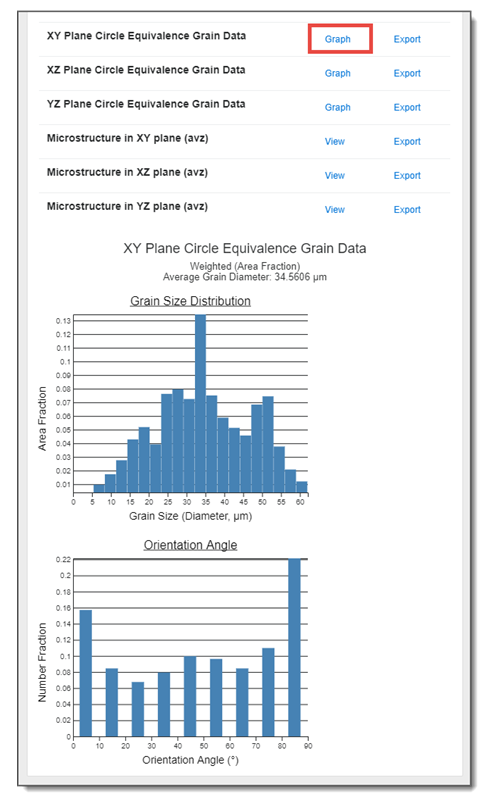
Grain area and diameter values for all the grains are aggregated into a Grain Size Distribution bar chart showing the area fraction of grains whose diameter falls in discrete ranges indicated on the chart. This bar chart is displayed in the application when you click the Graph link as shown in the following figure. While this particular bar chart is not exportable, the full data can be exported as a .csv file. The .csv file does not contain the same data as the aggregate bar charts but contains full data for each grain with area fraction and equivalent circle diameter such that you can produce similar graphs on your own. A second bar chart shows a similar aggregate of Orientation Angle.
From the charts below, this particular result set shows the majority of grains have a diameter between 30 and 35 microns and are oriented between 80 and 90°.
How Porosity is Revealed in Results
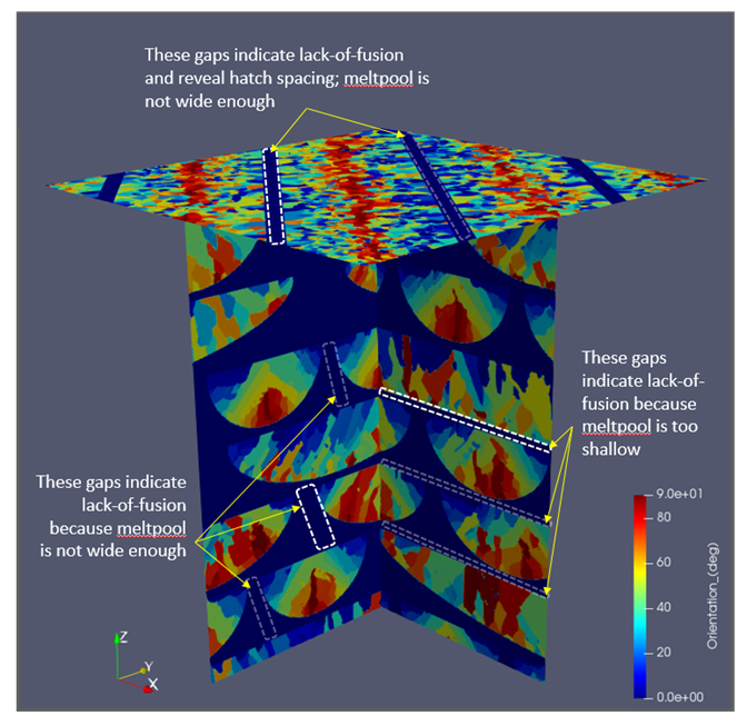
It is always wise to examine your results to be sure they make logical and intuitive sense and to enhance your understanding of the microstructural phenomena occurring in the simulation. Instances of lack-of-fusion porosity, in particular, are important to discern and are, in fact, easy to recognize in microstructure results. A grain number of 0 indicates a location of unmelted material, or lack-of-fusion porosity. Orientation and grain number maps will show gaps at these locations, as shown in the following figure. This example was run as an exaggerated case to show lack-of-fusion porosity by defining inputs such that the Melt Pool Depth was less than Layer Thickness, and Melt Pool Width was less than Hatch Spacing.
Evaluating Trends
When evaluating a material's microstructure, there is significant variability of results, even in tightly controlled experimental lab tests. This is why our validation process includes printing multiple test cubes, and why we recommend that you run at least three to five simulations using random seed numbers and average the results.
Confidence can be found in evaluating trends in the data. In general, you should see these trends in your Microstructure simulation results:
The lower the energy density put into the system, the smaller the resulting grain size. Energy density is the energy being put into the material at the melt pool location per unit volume. The most significant factors contributing to energy density are the laser power, scan speed, hatch spacing, layer thickness, and the material's absorptivity. So for a given material, to decrease the energy density you can decrease Laser Power, increase Scan Speed, increase Hatch Spacing, and/or increase Layer Thickness.
If the cooling rate increases, grain sizes should decrease.
If the average grain size is smaller, variation in grain size will also be smaller.