


In this simulation type, given a material, a part, and all the process parameters, melt pool dimensions and thermal history are output for a particular cross-section of your part, simulating results from a coaxial average sensor. This feature is a Beta feature at this release.
For your chosen machine and material, Single Bead simulations allow you to explore the effects of process parameter combinations on melt pool size and shape for a single scan line. Porosity simulations allow you to study lack-of-fusion porosity in a block of material for selected sets of process parameters. In a Thermal History simulation, you will gain insight into the thermal history of your own, unique part. Different thermal conditions may exist in different areas of your part, leading to hot and cold regions that may be indicative of hot cracking, delamination, porosity or property variations, among other things.
The Coaxial Average Sensor provides a map of the instantaneous melt pool dimensions (length, width, and depth) and average temperatures within a circular field of view (FOV) centered about the laser position at the top surface of the part. The output includes a single 2D set of .vtk data for each deposit layer within the height range(s) specified.
Select a part for simulation by adding it to your simulation form. Regardless of whether you add a part or a build file, it must have been uploaded first to the Parts Library or Build File Library, respectively.
Supports are not simulated in Thermal History simulations.
Select from the following materials available for Thermal History simulations:
17-4 PH stainless steel
316L stainless steel (Beta)
Aluminum Al357
Aluminum AlSi10Mg
Cobalt-chrome (CoCr)
Inconel 625
Inconel 718
Titanium 6-4
Specify the following process parameters:
Machine - A placeholder for future machine configurations. Defaults to Generic for now.
Baseplate Temperature (°C) - The controlled temperature of the baseplate. Must be between 20 and 500. The default value is 80°C.
Layer Thickness (μm) - The thickness of the powder layer coating that is applied with every pass of the recoater blade. Must be between 10 and 100. The default value is 50 microns.
Starting Layer Angle (°) - The angle at which the first layer will be scanned. It is measured from the X axis, such that a value of 0° results in scan lines parallel to the X axis. Must be between 0 and 180°. The starting layer angle is commonly set to 57° (default).
Layer Rotation Angle (°) - The angle at which the major scan vector orientation changes from layer to layer. Must be between 0 and 180°. This is commonly 67° (default).
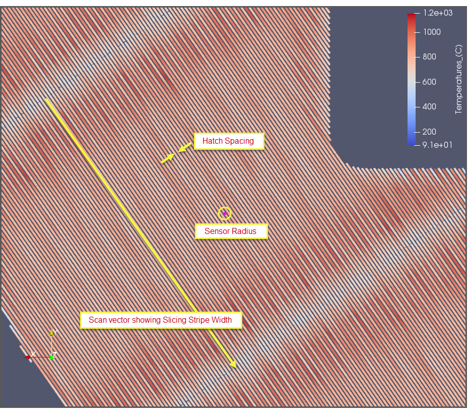
Hatch Spacing (μm) - The distance between adjacent scan vectors when rastering back and forth with the laser. Hatch spacing should allow for a slight overlap of scan vector tracks such that some of the material re-melts to ensure full coverage of solid material. Must be between 0.06 and 0.2 mm. The default Hatch Spacing is 0.1 mm (100 microns).
Slicing Stripe Width - When using the stripe pattern for scan strategy, the geometry can be broken up into sections, called stripes. The stripes are scanned sequentially to break up what would otherwise be very long continuous scan vectors. Slicing Stripe Width is commonly set to 10 mm wide. Memory requirements for the thermal solution will expand significantly as you increase the Slicing Stripe Width much beyond the default. Must be between 1 and 100 mm. Defaults to 10 mm.
Laser Beam Diameter (μm) - The width of the laser on the powder or substrate surface defined using the D4σ beam diameter definition. Usually this value is provided by the machine manufacturer. Sometimes called laser spot diameter. Defaults to 100 μm.
Laser Power (W) - The power setting for the laser in the machine. Must be between 50 and 700. Defaults to 195 Watts.
Scan Speed (mm/sec) - The speed at which the laser scans, excluding jump speeds and ramp up and down speeds. Must be between 350 and 2500. The default value is 1000 mm/sec.
The Outputs area of the simulation form is where you select which sensors to simulate. At this release, only a Coaxial average sensor is available.
The Sensor Radius defines the FOV radius over which the temperatures are averaged. As the thermal gradients are highest in the immediate proximity of the melt pool, the average temperature will generally decrease as the radius is increased. This allows you to observe the temperature field at multiple length scales. The melt pool dimensions are not averaged, and therefore unaffected by the FOV radius. The Sensor Radius must be between 0.05 and 15 mm. The default value is 1.0.
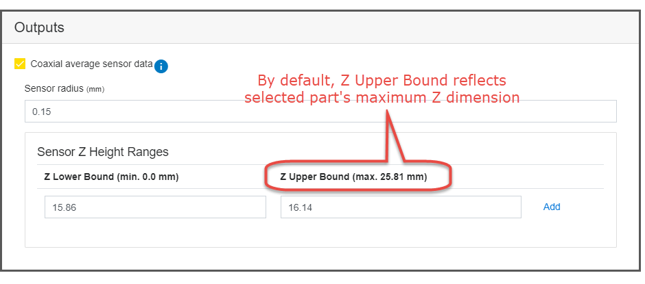
The Sensor Z Height Range controls which layers in the part will have results generated. Values are relative to the bottom of the part (Z=0). Use a height range of the area of the part that is of interest, such as at the height of a special geometric feature. When you have a part selected in the simulation form, the Z Upper Bound reflects that part's maximum height dimension, in millimeters.
As an example, say you have a part where the location of interest is around 16 mm. If you have a Layer Thickness of 35 microns, a Sensor Z Height Range of 15.86 (lower bound) to 16.14 (upper bound) will produce 8 ((16.14-15.86)/.035) layers of results files. (Note that you do not need to specify a range that will produce an even multiple of layers.)
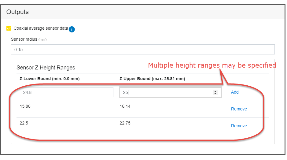
Multiple sets of ranges may be specified. Add each new range to the form, as needed. The simulation time will increase as the total combined height selected increases.
Results for Thermal History simulations consist of 2D .vtk files, one for each layer specified in the height range. The position of each data point corresponds to the laser position at each finite time step as the layer was scanned. As a result, the data will appear as thin lines that represent the laser's scan path.
Paraview is an open-source, multi-platform data analysis and visualization application. Within Paraview, extract the melt pool and temperature data by doing the following:
Open a file corresponding to a layer and make it active.
Select a data type to display, such as melt pool depth, length, width, or temperatures. (Remember, temperatures are averaged over the FOV.)
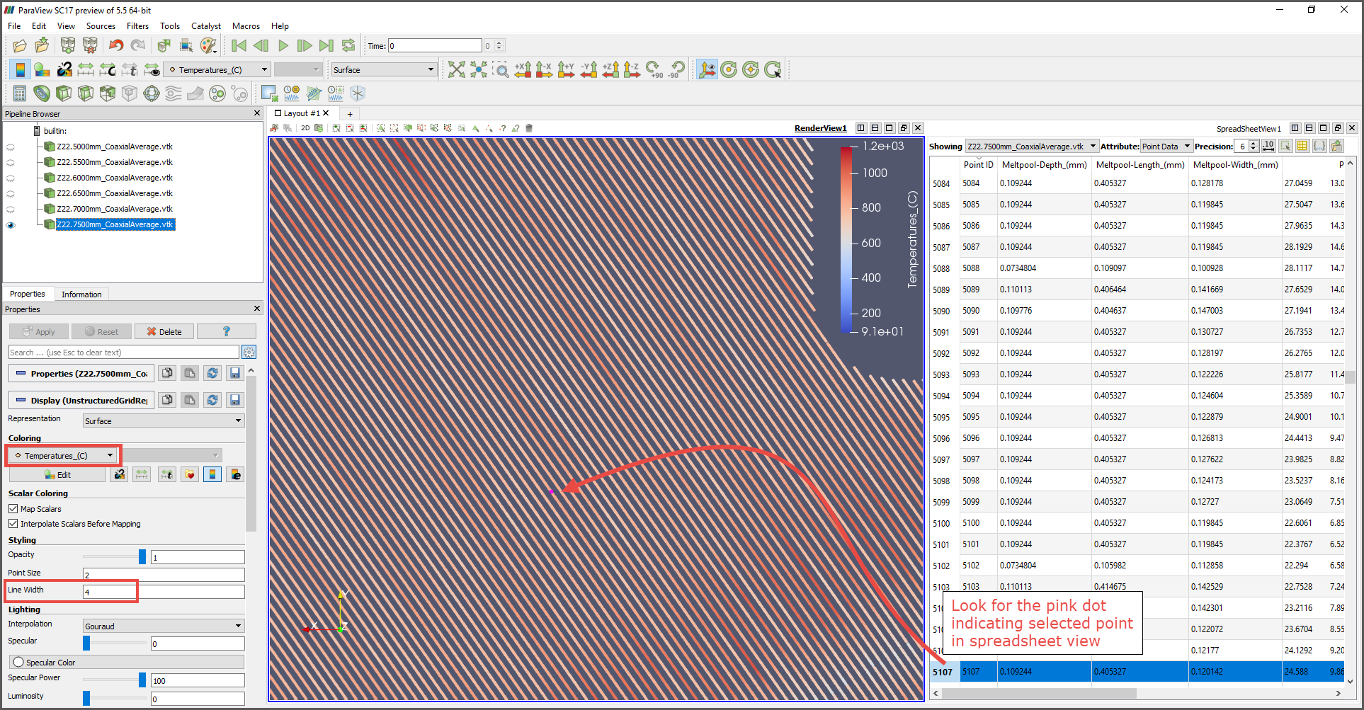
Set up two side-by-side windows so you can view the rendered results in one window and a spreadsheet view of the data in the other.
In the render view window, increase the line width to improve visibility.
In the spreadsheet view window, select any point and then press and hold the down-arrow key down to jump through data points so as to "follow the dot" in the render view window. This gives you a visualization of how the laser is scanning that cross section of the part.
In the render view window, zoom in and out, as desired, to examine your results.
When reviewing results, you may want to zoom out to see the entire cross-section and look for hot and cold spots in various geometric features on different layers. That gives you an indication for how the specific scan pattern you've selected results in a specific thermal distribution (which may or may not differ significantly from layer to layer depending upon the scan pattern and geometry combination).