


The solution of Equation 5–14 is found with the finite difference method. The differential equation represents a linear second order boundary value problem.
 | (5–15) |
where the derivatives are replaced with

|

|
where  are the displacements at the supporting
points through the thickness and
are the displacements at the supporting
points through the thickness and  is the distance
between two consecutive supporting points. Their placement scheme
for a single-layer laminate is shown on the left of Figure 5.5: Integration Scheme. The boundary conditions lead to a non-singular
linear system of equations (LSoE) and are represented by the INS which
have to vanish at the top and bottom surfaces of the laminate.
is the distance
between two consecutive supporting points. Their placement scheme
for a single-layer laminate is shown on the left of Figure 5.5: Integration Scheme. The boundary conditions lead to a non-singular
linear system of equations (LSoE) and are represented by the INS which
have to vanish at the top and bottom surfaces of the laminate.
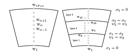
The above figure shows single layer (left) and multilayer laminate
(right) where the indices 1, 2, and 3 count the layers and  refers
to
refers
to  .
.
The through-the-thickness INS distribution is obtained by combining Equation 5–8 and Equation 5–10.
 | (5–16) |
This equation can be transformed to:
 | (5–17) |
and is integrated in the LSoE where  and
and  modify
the first and the last row of the left and right side of the LSoE,
respectively.
modify
the first and the last row of the left and right side of the LSoE,
respectively.
Every additional layer leads to two more interface continuity conditions that have to be fulfilled:
 | (5–18) |
The first derivative of the through-the-thickness displacements is found
using Equation 5–16. Additional supporting points, which
are placed outside the layer, are necessary to evaluate the INS at
the layer intersections. An integration scheme for a three layer laminate
is plotted on the right of Figure 5.5: Integration Scheme where the supporting
points n = [7,8,15,16] guarantee the through-the-thickness continuity
of the INS.
is found
using Equation 5–16. Additional supporting points, which
are placed outside the layer, are necessary to evaluate the INS at
the layer intersections. An integration scheme for a three layer laminate
is plotted on the right of Figure 5.5: Integration Scheme where the supporting
points n = [7,8,15,16] guarantee the through-the-thickness continuity
of the INS.