


During the simulation, the unit cells are laid one by one on the surface of the model to ensure full contact with the surface. The simulation starts from a given seed point and progresses in the given draping direction. In this phase, each draping cell initially has two known node points. Draping cells are laid until the model edge is reached. Then, the procedure is repeated in the opposite direction (if applicable) and in the orthogonal directions as shown below in Figure 5.1: Draping Scheme . After the main draping paths have been determined, the cells with three known nodes are populated. The algorithm resolves if the whole model is draped or if there are areas where the draping simulation needs to be restarted..
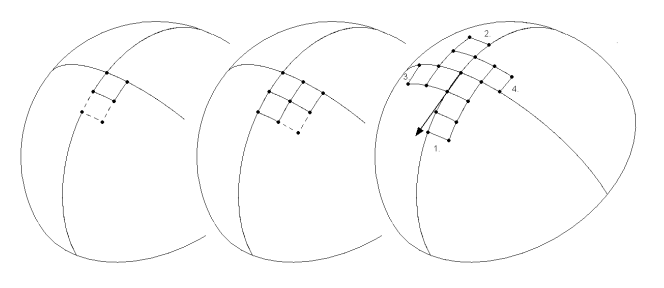
Note: Above figure represents draping of a cell that has two (left) or three (middle) known node points and propagation scheme using orthogonal directions (right).
The draping procedure involves the search for two types of draping cells: those with two known nodes or three known nodes as shown above. When two node points are known and the locations of the other two must be determined, the search algorithm is based on the minimization of the shear strain energy [ 4 ]:
 | (5–1) |
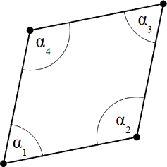
where G is the elastic shear modulus of the uncured reinforcement. The shear deformation is related to the angle α between the originally orthogonal fibers [ 3 ]:
 | (5–2) |
The total shear strain energy of the draping cell is defined as the sum of energy computed at the four corners. The two constants can be excluded and the minimization problem becomes:
 | (5–3) |
From this, the locations of the two node points can be determined with an iterative minimization algorithm. In the case of three known points, the search algorithm seeks the fourth node point in different ways depending on the material model in use.