ACP provides a multitude of post-processing analyses. The following instructions will help you get started in examining the results.
In Ansys Workbench, you can choose one of two methods to post-process results for composite materials: You can do it directly in Mechanical by adding a Composite Failure Tool, or you can add an ACP (Post) cell into the project schematic. This tutorial will cover post-processing through ACP (Post). Later tutorials explain post-processing in Mechanical.
Return to Workbench and drag an ACP (Post) system onto the ACP (Pre) system.

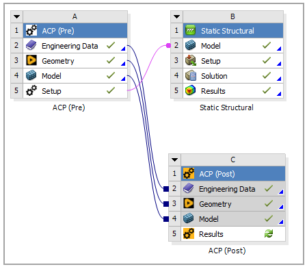
Drag and drop the Solution cell of the Static Structural system to the Results of ACP (Post).
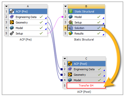
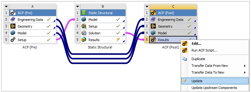
Update the Results cell of ACP (Post). Then, double-click Results to open ACP.
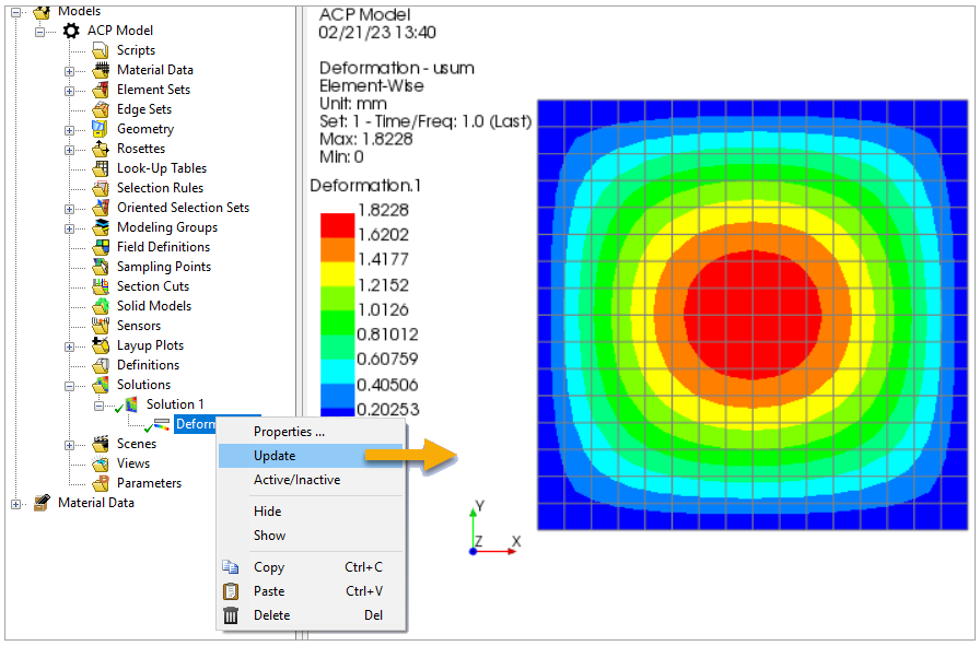
A deformation plot displays the panel's behavior for a specific solution. To create the panel's deformation plot, follow these steps:
In ACP, click the Update icon to update the project.
In the Tree, right-click Solution 1 under Solutions and select Create Deformation Plot to visualize the deformations.
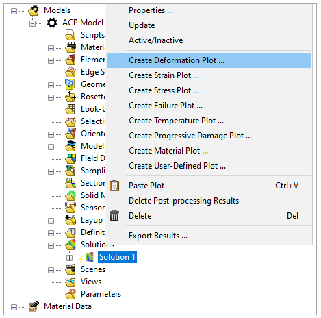
When the Deformation dialog appears, accept the defaults, and click OK.
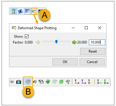
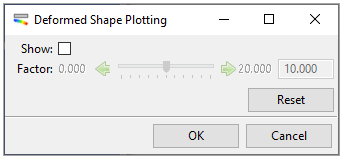
In the toolbar, set the deformation scale (A, below) and toggle mesh (B).
Update the entire project to visualize the plot.
Note: To show the plot, ensure that the Show Surface icon is deselected in the toolbar.
Failure criteria evaluate the strength of a composite structure. ACP (Post) provides a number of analyses to assess the strength assessment of a composite. It allows you to create failure definitions, then combine and configure them.
In this step, a combined Failure Criteria is configured to create an overall failure plot of the composite structure. The stress limits for your two materials were defined in the Engineering Data at the beginning of this tutorial. Before you begin, ensure that your material models contain the appropriate failure parameters. Then, create the failure plot:
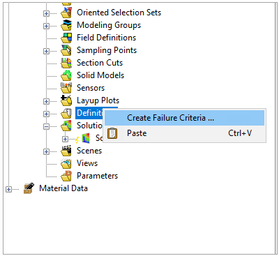
Right-click Definitions in the Tree and select Create Failure Criteria.
In the Failure Criteria Definition dialog, select Max Stress and Tsai-Wu under the Reinforced Ply Criteria tab. Select Core Failure under the Sandwich Criteria tab.
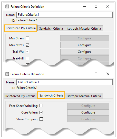
Click OK.
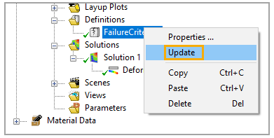
Right-click the Failure Criteria object and select Update.
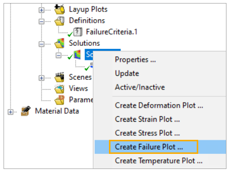
Right-click Solution 1 and select Create Failure Plot.
In the Failure Plot dialog, specify the following options as shown in the image below:
Under Scoping, select Entire Model (default).
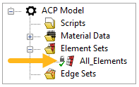
Tip: To customize the Data Scope, deselect the Entire Model. Then put the cursor in the Data Scope field and click an element set in the Tree View.
For Failure Criteria Definition, select FailureCriteria.1 from the dropdown menu.
Enable Show Critical Failure Mode and Show Critical Layer.
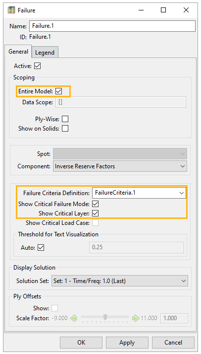
Click OK.
Hide the deformation scale by clicking on its toolbar icon and deselecting Show.
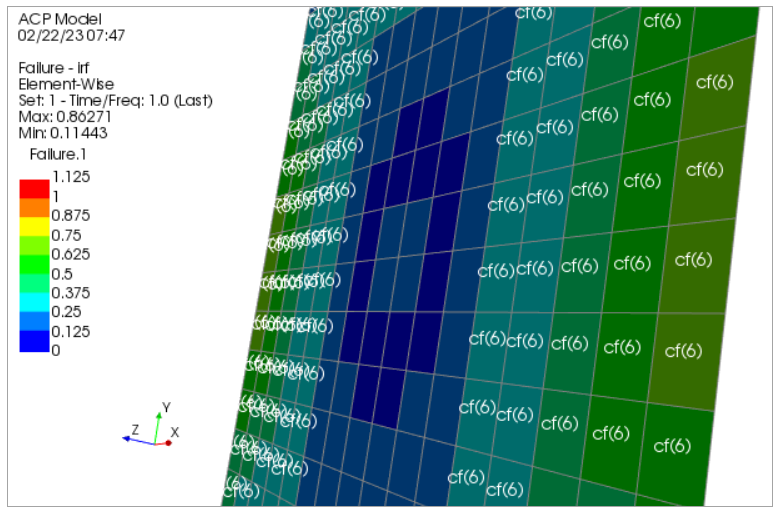
Update the model to see the overall failure plot:
The contour plot shows the maximum inverse reserve factor of each element (through all layers, selected failure criteria, and integration points).
The text plot indicates the critical layer (numerical value) and the critical failure mode (text value).
Tip:
 This icon in the toolbar labels the minimum and maximum
values on the plot.
This icon in the toolbar labels the minimum and maximum
values on the plot.
A stress plot is a post-processing solution that displays stress values at the bottom, mid or top position of the ply and at the element center (or at the bottom or top of the laminate if ply-wise is disabled).
Right-click Solution 1 and select Create Stress Plot.
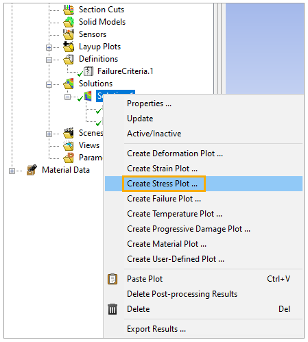
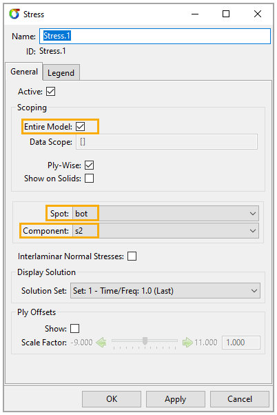
Set the scope to the Entire Model, as a Ply-Wise stress plot for the transverse stresses. Select bot for the Spot and s2 as the Component.
Click OK.
Update the project.
Click any Analysis Ply to see its stress distribution. Ply-wise plots are only visible when a ply is selected.

A through-the-thickness plot is one of the post-processing analyses of a sampling point. It shows the through-the-thickness distribution of strains, stresses, or failure results.
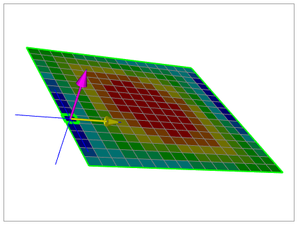
Sampling Points are used in post-processing to access ply-wise results. ACP samples through the specific element near the given coordinates to run detailed analyses (lay-up plots, through-the-thickness plots, and laminate engineering constants).
The through-the-thickness results can be visualized in the Analysis tab of the Sampling Point. To view the through-thickness plot:
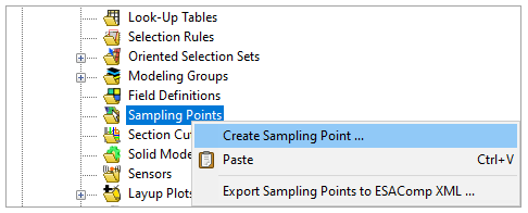
Right-click Sampling Points and select Create Sampling Point.
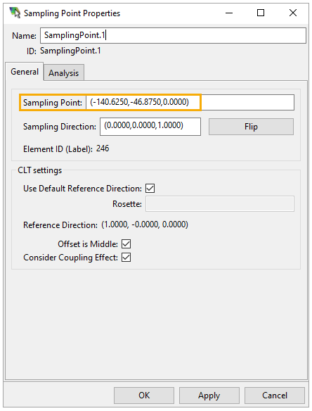
Set the coordinates of your Sampling Point and then click Apply.
In the Analysis tab, set the properties as shown in the figure below.
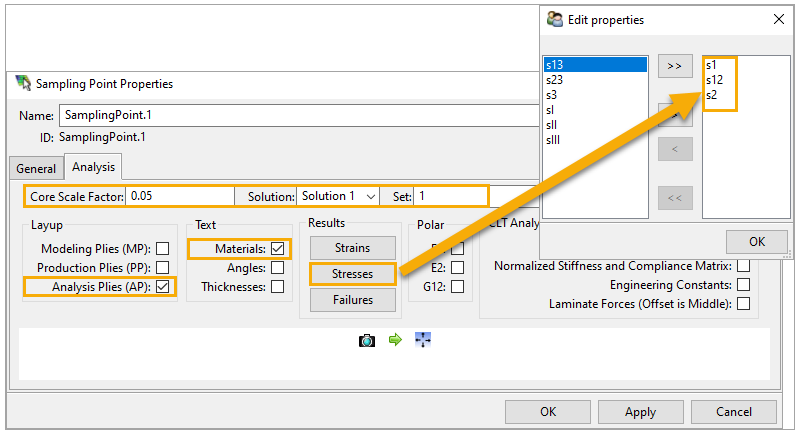
Click Apply to visualize the through-the-thickness plot in the same dialog.
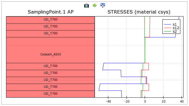
Select any analysis ply of the Sampling Point to visualize the stress distribution of a single ply.