


The homogenization methods in Material Designer account for the individual properties of the fiber and resin constituents as well the microstructure through the fiber aspect ratio and orientation. However, several complex factors can impact these material properties: The bonding agents added during injection have a significant influence on the properties of the composite. Fiber breakage is likely to occur during the mixing process. And deviations from the nominal fiber aspect ratio can be expected.
Another factor that must be considered is the nonlinear deformation behavior of short fiber reinforced composites– a result of the highly nonlinear behavior of the resin, interface debonding, and micro-crack formation during manufacturing and subsequent loading. All these factors vary according to the manufacturing process used. Clearly, experimental data is required to accurately model these kinds of materials.
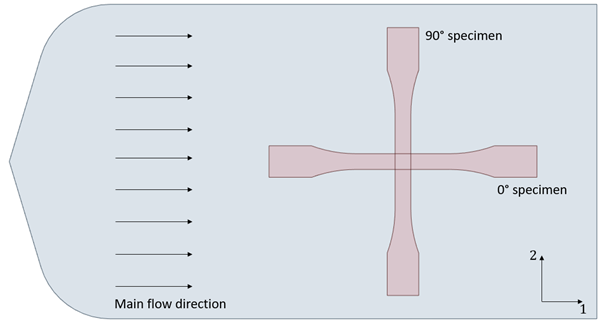
Specifically, stress-strain curves from uniaxial tension experiments must be collected from two specimens milled out of an injection molded plate: one at 0° and another at 90° degrees with respect to the main flow direction (see the figure below). Tests and specimens should be prepared in accordance with the ISO 527 or the ASTM D638 standard in quasi-static conditions.
Also, it is safe to assume the average second-order fiber orientation tensor in the injection molded plate is known. You can obtain the fiber orientation field by microscopic computed tomography (CT) scans or by injection molding simulation.
Use the following procedure to enter and store experimental data for short fiber composites in Material Designer:
In Material Designer, right-click Experimental Data and create a new Dataset.
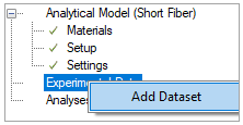
A new dialog will open:
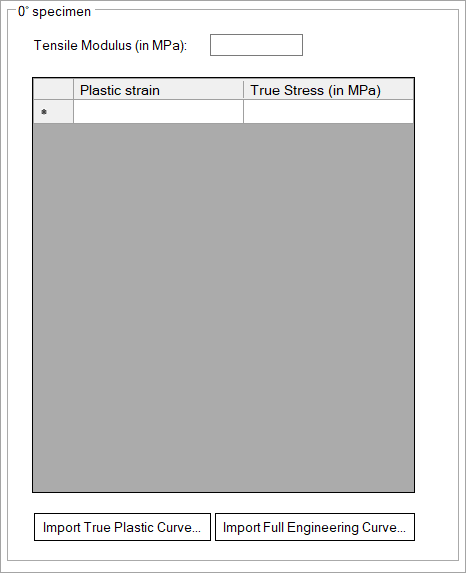
Enter experimental data using either of the two following approaches:
Loading the true plastic strain and stress using the button.
From the measured engineering stress-strain curves of the 0° and 90° specimens, extract the tensile modulus and prepare the true-stress versus plastic-strain curves. To this end, recall the following relations between engineering and true stress and strain: 
(2–1)
Plastic strain is then given by 
(2–2)
where  is the plastic strain and
  is the (experimental) Young’s modulus.
(This calculation can be easily done in a spreadsheet.)
is the (experimental) Young’s modulus.
(This calculation can be easily done in a spreadsheet.) Loading the full engineering strain and stress curve using the button.
You can import the full engineering stress and strain curve without considering the definition of the elastic or plastic segments. The software internally computes the conversion to true quantities, the calculation of the Young's modulus, and the definition of the plastic strain and stress curve. This approach follows the one in [Dillenberger (2020)], with an additional optimization of the initial strain offset for a more accurate determination of the yield point. In particular, the software first calculates the Young's modulus via fitting the values of the imported curve in the strain region between 0.05% and 0.25% using linear regression. Therefore, a straight line can be drawn between a certain value of strain offset  and the computed Young’s modulus such that
it intercepts the original stress strain curve. The found
interception defines the yield point. The strain values are then
corrected using the equation:
and the computed Young’s modulus such that
it intercepts the original stress strain curve. The found
interception defines the yield point. The strain values are then
corrected using the equation:
(2–3)
where  is defined as:
(2–4)
with 

 is the strain at the last point of the stress
strain curve.
is the strain at the last point of the stress
strain curve.After the strain is corrected, the plastic strain is calculated accordingly using the method defined in approach a. Once the calculation finishes, a dialog opens displaying the reconstructed curve on top of the experimental one: 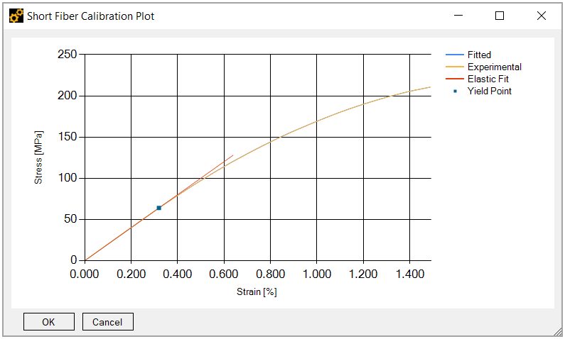
If you hover the mouse over the yield point, the computed yield strain and stress as well as the Young's modulus are shown: 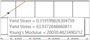
Click the button to store the calibration in the appropriate table (0° or 90° data) or click to discard the computed quantities.