


Creating a Polar Intensity Sensor
This page shows how to create an Intensity Sensor that computes and analyzes radiant or luminous intensity following standard and intensity formats (IESNA format, Eulumdat format).
To create a Polar Intensity Sensor:
-
From the Light Simulation tab,
click Intensity
_Sensor_Polar_Intensity.png) .
.
-
In General, from the
Type drop-down list:
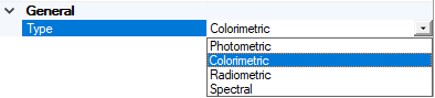
Select Photometric if you want the sensor to consider the visible spectrum and get the results in cd.
Note: In case of a photometric result generation, the International Commission on Illumination (CIE) defines the visible spectrum as follows: "There are no precise limits for the spectral range of visible radiation since they depend upon the amount of radiant flux reaching the retina and the responsivity of the observer. The lower limit is generally taken between 360 nm and 400 nm and the upper limit between 760 nm and 830 nm".Select Radiometric if you want the sensor to consider the entire spectrum and get the results in W/sr .
Note: With both Photometric and Radiometric types, the illuminance levels are displayed with a false color and you cannot make any spectral or color analysis on the results.Select Colorimetric to get the color results without any spectral data or layer separation (in cd or W/sr).
Select Spectral to get the results and spectral data separated by wavelength (in cd or W/sr).
Note: Spectral results take more time to compute as they contain more information.
-
From the Format drop-down
list, select the type of standard you want to follow:
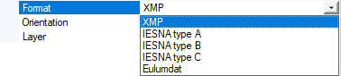
Select IESNA type A, B or C if you want to generate an .ies file and follow US standard data format for storing the spatial light output distribution.
Select Eulumdat if you want to generate an .ldt file and follow the European standard data format for storing the spatial light output distribution.
-
From the Layer drop-down
list:
Select None to get the simulation's results in one layer.
Select Source if you have created more than one source and want to include one layer per active source in the result.
Tip: You can change the source's power or spectrum with the Virtual Lighting Controller in the Virtual Photometric Lab or in the Virtual Human Vision Lab.Select Face to include one layer per surface selected in the result.
Tip: Separating the result by face is useful when working on a reflector analysis.In the 3D view click
_Sensor_Contributing_Faces.png) and select the
contributing faces you want to include for layer separation.Tip: Select a group (Named Selection) to separate the result with one layer for all the faces contained in the group.
and select the
contributing faces you want to include for layer separation.Tip: Select a group (Named Selection) to separate the result with one layer for all the faces contained in the group.Select the filtering mode to use to store the results (in the *.xmp map):
_Sensor_Filtering_Mode.png)
Last Impact: with this mode, the ray is integrated in the layer of the last hit surface before hitting the sensor.
Intersected one time: with this mode, the ray is integrated in the layer of the last hit selected surface if the surface has been selected as a contributing face or the ray intersects it at least one time.
Select Sequence to include one layer per sequence in the result.
-
Set the Axis System of the
sensor:
If you selected IESNA type B, click
_Origin_Point.png) to select an origin,
to select an origin, _Sensor_Axis_X.png) to select a line to define the
Polar Axis and
to select a line to define the
Polar Axis and _Sensor_Axis_Y.png) to select a line to define VO Axis.
to select a line to define VO Axis. If you selected IESNA type A, IESNA type C or Eulumdat, click
to select an origin, to select a line to define the
Polar Axis and to select a line to define HO Axis.
Note: If you define manually one axis only, the other axis is automatically (and randomly) calculated by Speos in the 3D view. However, the other axis in the Definition panel may not correspond to the axis in the 3D view. Please refer to the axis in the 3D view. -
If you want to bring the measuring field of the sensor closer to the
source, in Properties set Near field to True.
The near-field sensor appears in the 3D view.
Note: If Near field is deactivated, the intensity is located at the infinite.The results obtained with a near-field sensor can be inaccurate on the edge of the map, over a width equal to the radius of a cell.
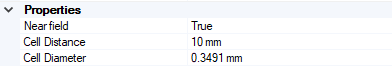
In Cell Distance, define the position of the sensor in regard to the origin in the 3D view.
In Cell Diameter, define the actual size of the photosensitive sensor. The size must be superior to one pixel.
-
In Optional or advanced
settings
_Speos_Options.png) :
:
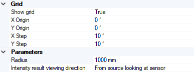
If needed, adjust the preview of the grid by editing the values.
If you want to adjust the position preview of the sensor, change the radius (in mm).
From Intensity result viewing direction, define where the sensor is placed regarding to the source:
Select From source looking at sensor to position the observer point from where light is emitted.
Select From sensor looking at source to position the observer in the opposite of light direction.
The intensity sensor is created and is visible both in Speos tree and in the 3D view.