The Icepak Solve Setup Dialog (Transient)

A solution setup includes the settings you need to define for the Icepak simulation. For transient simulations, the Icepak Solve Setup dialog box contains the following tabs:

• General
• Save Fields
• Simulation Control (Dynamic Thermal Modeling Beta)
• Convergence
• Solver Settings
• Radiation
• Solar Radiation
• Defaults

Click here for scripting information related to this feature.

The Solve Setup Defaults drop-down list contains the following options that automatically configure settings based on your selection. See Transient Icepak Solve Setup Defaults for more information.

• Solve Setup Defaults
• Forced Convection Defaults
• Natural Convection Defaults
• Mixed Convection Defaults
• Conduction Only Defaults
• LTI ROM Defaults

Name	The Name of the setup appears in the Project Manager window.
Maximum Number of Iterations (Steady State only)	Maximum Number of Iterations is the number of solution iterations to be performed in a simulation. The simulation will stop when these iterations have been performed or the Convergence Criteria are satisfied, whichever happens first. For relatively simple models, the default of 100 should be sufficient for the solution to converge, but for more complex models you may need to increase this value.
Enabled	The Enabled check box disables/enables a setup. Only enabled setups are run when you select Analyze All.
Transient Setup (Transient only)
Start	Start defines the start time for the simulation.
Stop	Stop defines the ending time for the simulation.
Time Step	Time Step defines the duration of a time step. To define varying time steps, enable the check box to open the Advanced Time Variations dialog box. See Specifying Varying Time Steps for Transient Solution Setups for more information.
Advanced	Click Advanced to open the Advanced Time Variations dialog box. See Specifying Varying Time Steps for Transient Solution Setups for more information.
Iterations/Time step	Iterations/Time step defines the maximum number of iterations to be performed per time step. If the convergence criteria are satisfied before this number of iterations is performed, the simulation advances to the next time step. The default value of 20 iterations/time step should be acceptable for most cases. If you find that the solution is not converging at each time step, you can increase Iterations/Time step value and/or decrease Time Step.
Preview	Click Preview to display the Variations Preview dialog box, which contains a preview of all transient advanced time variations in the design.
Problem Types
Temperature	When enabled, the Temperature check box instructs the solver to include thermal calculations in the analysis.
Flow	When enabled, the Flow check box instructs the solver to include fluid calculations in the analysis.
Flow Regime
Laminar	Laminar flow is smooth, regular, deterministic, and steady. In laminar flow, fluid mixing and heat transfer take place on a molecular level. The molecular (or dynamic) viscosity and the thermal conductivity are the quantities that measure the amount of mixing and heat transfer. Laminar is the default flow regime.
Turbulent	Turbulent flows are characterized by fluctuating velocity fields. In turbulent flow, the degree of fluid mixing and heat transfer is much greater than in laminar flow, and takes place on a global, or macroscopic, level rather than on a molecular level. The amount of fluid mixing is measured by an effective viscosity, which is the sum of the dynamic viscosity and the turbulent eddy viscosity. If you select Turbulent, click Options to open the Turbulent Flow Model dialog and select a model. The default turbulent flow model is Zero Equation.
Radiation Model
Off	Off disables radiation for the solution. Off is the default setting.
Discrete Ordinates	The Discrete Ordinates (DO) radiation model solves the radiative transfer equation (RTE) for a finite number of discrete solid angles, each associated with a vector direction fixed in the global Cartesian system (x, y, z). The DO model solves for as many transport equations as there are directions . The solution method is identical to that used for the fluid flow and energy equations.
Ray Tracing	With the Ray Tracing radiation model, the ray paths are calculated and stored prior to the fluid flow calculation. At each radiating face, rays are fired at discrete values of the polar and azimuthal angles. To cover the radiating hemisphere, is varied from 0 to and from 0 to . Each ray is then traced to determine the control volumes it intercepts as well as its length within each control volume. This information is then stored in the radiation file (.s2s.gz), which is then read in before the fluid flow calculations begin.
Include Gravity	To include the effect of gravity in the simulation for natural convection models, select Include Gravity. Define the gravity vector settings in the Icepak Design Settings. Natural convection models require Include Gravity to be enabled.
HPC and Analysis Options	High performance computing (HPC) enables a range of different technologies in Icepak that allows efficient simulation of extremely large and complex problems. See High Performance Computing for more information.

Field Save Times (Transient only)
None	None specifies that Icepak field quantity data will not be saved at any interim time points during the simulation.
Every # Steps	Every # Steps specifies the frequency at which Icepak field quantity data is saved for creating post-processing (fields calculations, plots, reports, etc.). The amount of save times is determined by the simulation start and stop times and duration of a time step defined on the General tab.
Varying	Varying displays the Save Field - Transient Variation dialog box, in which you can specify varying save times using a piecewise constant variation function. Click Edit to make changes to the variation function.

Control Program (Dynamic Thermal Modeling)
Use Control Program	Use Control Program allows you to select the Program script you previously created using the Thermostat for Source Control toolkit.

Flow	These settings are the solution-residual values used to determine convergence. Solution residuals measure the error or imbalance in the conservation equations that Icepak solves. When all solution residuals are less than or equal to their specified convergence criteria, the solution will be considered converged. Turbulent Kinetic Energy, Turbulent Dissipation, and Specific Dissipation Rate are enabled by the selection of certain turbulent flow models. Discrete Ordinates is enabled if the Radiation Model is set to Discrete Ordinates. Joule Heating is enabled if the power for a block boundary condition is defined as joule heating.
Energy
Turbulent Kinetic Energy
Turbulent Dissipation
Specific Dissipation Rate
Discrete Ordinates
Joule Heating

Initial Conditions
X, Y, Z Velocity	These settings specify the initial conditions for the fluid in the flow region. The initial conditions are the initial guess for the various solution fields used by the solution procedure. Turbulent Kinetic Energy, Turbulent Dissipation, and Specific Dissipation Rate are enabled by the selection of certain turbulent flow models.
Temperature
Turbulent Kinetic Energy
Turbulent Dissipation
Specific Dissipation Rate
Use Model Based Flow Initialization	Use Model Based Flow Initialization instructs the Electronics Desktop to automatically evaluate inlet and outlet conditions to use optimal values for solution variables.
Import Options
Mesh	Mesh allows to use mesh from an existing Icepak design and is automatically enabled after using the Add a Mesh Linked Solution Setup option. Mesh from the selected design is imported and used in the simulation. The mesh from the source design must conform to the target design's model geometry. Seeing Importing Mesh for more information.
Start/Continue...	Start/Continue from a previously solved setup allows you to begin or resume a simulation from a design you have previously solved. See Transient Import Options Requirements for more information.
Note: If the design has a mesh link and solve setup link, if you remove the solve setup link, the mesh link is not automatically removed.
Frozen flow simulation	Frozen flow simulation allows you to disable the flow of the linked steady-state or transient design. If enabled, only the energy equation is solved during the analysis. If the linked solution did not solve for flow, this option is not active.
Use end time from source (Transient only)	Use end time from source allows you to start the analysis from the linked solution's stop time. For example, if the linked solution solved from 0 to 10 seconds and the target solution is set to solve from 0 to 20 seconds, the target solution starts solving at 10 seconds and stops at 20 seconds.
Copy fields from source (Transient only)	When Use end time from source is enabled, Copy fields from source is available. Enable this option to copy fields data from the source design to make it available for post-processing in the target design. Using the example in the definition above, fields data from the target design (from 0 to 10 seconds) will be available to post-process in the target design.
Advanced Options	Click Advanced Options to display the Advanced Solver Settings dialog box. To review advanced solver settings, see The Icepak Solve Setup Dialog.

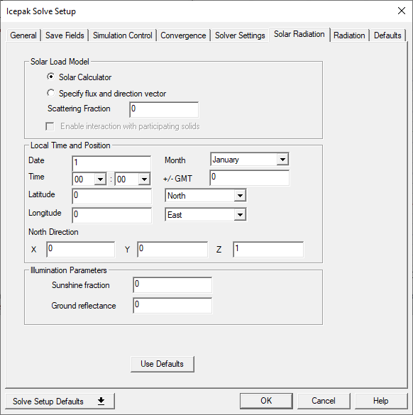
Solar Load Model
Solar Load Model	Select Solar Calculator to compute the solar radiation based on time and geographic parameters or Specify flux and direction vector to specify solar radiation values and a solar radiation direction vector.
Scattering Fraction	Scattering Fraction specifies the amount of direct solar radiation that is reflected from opaque objects in your model. The reflected radiation is evenly distributed among all objects that participate in solar loading.
Enable interaction with participating solids	When Discrete Ordinates is defined as the radiation model, select Enable interaction with participating solids to model the solar irradiation as discrete ordinate fluxes at the global region boundaries. This allows semi-transparent walls and participating solids to absorb, refract and scatter the incident solar irradiation.
Local Time and Position (Solar Calculator)
Date and Month	Specify a Date and Month.
Time	Time specifies the local time at the desired location. Select the hour and minute from the drop-down lists. The time is based on a 24-hour clock, therefore acceptable values range from 0 h 0 min (12:00 a.m.) to 23 h 59 min (11:59 p.m.).
+/- GMT	+/- GMT specifies the local time zone of the desired location. If the time you enter is a local time, specify the current time zone by providing the offset in the +/- GMT entry. If the time you enter is already in GMT, then +/- GMT should be set to 0 (zero). For example, enter -5 to specify Eastern Standard Time (EST).
Latitude	Specify the Latitude of the desired location. Values can range from -90° (the South Pole) to 90° (the North Pole), with 0° defined as the equator. Select the hemisphere (N or S) from the menu to the right of the Local Longitude entry field.
Longitude	Specify the Longitude of the desired location. The longitude is approximated if you specify the local time zone, but you can enter a more precise value if you know it. Any value you enter here will take precedence over the time zone. Values may range from 0° to 180°. Select the hemisphere (W or E) from the menu to the right of the Local Longitude entry field.
North Direction Vector	The North Direction Vector specifies the northward direction relative to the model. Enter the appropriate values in the X, Y, and Z fields. The default northward direction is in the Z direction.
Illumination Parameters (Solar Calculator)
Sunshine fraction	Sunshine fraction is a factor between 0 and 1 used to account for the effects of clouds that may reduce the direct solar irradiation. Clear sky is modeled by setting the value equal to 1 and complete cloud cover is modeled by setting the value equal to 0. Partial cloud cover is modeled by setting the value to be between 0 and 1. The default value is 1.0.
Ground reflectance	Ground reflectance is a parameter that is used in determining the contributions of reflected solar radiation from ground surfaces. Reflected solar radiation from ground surfaces is a function of the direct normal irradiation, the time of the year, the tilt angle of the surface, and the ground reflectance. If is treated as part of the total diffuse solar irradiation. Ground reflectance values can vary depending on the ground surface (that is, concrete, grass, rock, gravel, asphalt). The default value is 0.2.
Solar Flux and Direction Vector
Direct solar irradiation	Direct solar irradiation specifies the amount of energy per unit area due to direct solar irradiation. This value may depend on the time of the year and the clearness of the sky.
Diffuse solar irradiation	Diffuse solar irradiation specifies the amount of energy per unit area due to diffuse solar irradiation. This value may depend on the time of year, the clearness of the sky, and also on ground reflectivity.
Solar Direction	Solar Direction specifies the direction of solar irradiation relative to the model. Enter the appropriate values in the X, Y, and Z fields.

Iteration Parameters
Flow Iterations per Radiation Iteration	The Flow Iterations per Radiation Iteration parameter is set to 1 by default. This implies that the radiation calculation is performed once every iteration of the solution process. Increasing the number can speed the calculation process, but may slow overall convergence.
Maximum Radiation Iterations (Ray Tracing only)	The Maximum Radiation Iterations controls the maximum number of iterations of the radiation calculation during each global iteration.
Angular Discretization (Discrete Ordinates only)
Theta and Phi Divisions	Theta Divisions () and Phi Divisions () will define the number of control angles used to discretize each octant of the angular space. A finer angular discretization can be specified to better resolve the influence of small geometric features or strong spatial variations in temperature, but larger numbers of Theta Divisions and Phi Divisions will add to the cost of the computation.
Theta and Phi Pixels	Theta Pixels and Phi Pixels are used to control the pixelation that accounts for any control volume overhang. For problems involving gray-diffuse radiation, the default pixelation of 1 × 1 is usually sufficient. The computational effort, as a result of increasing the pixelation, is less than the computational effort caused by increasing the divisions. However, increasing the pixelation does add to the cost of computation.
Cluster Parameters (Ray Tracing only)
Faces per Surface Cluster	Faces per Surface Cluster controls the number of radiating surfaces. By default, each is set to 20, so the number of surface clusters (radiating surfaces) will be equal to the total number of surface mesh elements divided by 20. For larger problems, you may want to reduce the number of surface clusters by increasing the faces per surface cluster to reduce both the size of the view factor file and the memory requirement. Such a reduction in the number of clusters, however, comes at the cost of some accuracy. The surfaces that are not adjacent to fluid regions will not participate in radiation.
View Factor Parameters (Ray Tracing only)
Resolution	Increasing Resolution helps reduce the numerical errors caused by the finite-resolution approach used to compute the projected areas of the surface clusters and the resulting view factors. By default, it is set to 5. In most cases, however, the default settings will be sufficient.