Assigning Arrays in HFSS

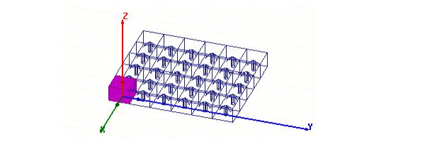
HFSS permits you to assign a virtual array based on a unit cell object, which can be a native design, a 3D component, or a SBR+ Parametric Antenna. For driven Modal and driven Terminal designs for HFSS with Hybrid and Arrays Solution Types, you can then simulate the array model using distributed processing, treating the instances as parent and child objects. This permits faster definition, display, and simulation of array based designs, such as antenna arrays. You can plot and animate array fields on cutplanes, lines or points. Post processing lets you view fields on any virtual instance.

The unit cells for an array can be rectangular, parallelogram, or hexagonal. HFSS SBR+ allows you to create Parametric Arrays from any of the parametric antennas. You can define the required primary and secondary boundaries so as to create offset arrays. You can only edit the settings in the physical cell and these settings will be applied to the corresponding instances in the virtual cells.

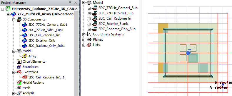
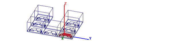
You can also create 3D components from unit cells, and use them to create a 3D Component Array.

Once you have defined an array, you can designate any cell in the array as active or passive, or as padding. You can use the padding cell designation to define arbitrarily irregular arrays. Cells designated as padding are treated as background material for fields calculations.

Most boundaries and excitations defined in the physical unit cell will have their corresponding instances in each virtual cell. The exception is incident wave, which is applied across the whole model and should include the 'expanded' model based on the array setup.

Components can now have different bounding box sizes (i.e., non-uniform sizing). In addition, HFSS supports arbitrary-sized internal air paddings, allowing flexibility for minor adjustments to existing arrays. However, to maintain array integrity, the array must remain perfectly tiled.

A Beta Feature allows you to have Multiple Component arrays in an HFSS design.

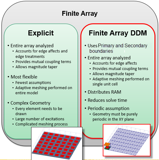
When the target design is a finite array, having both enforced E and enforced H options is not allowed. For all analytic incident waves except plane wave such as Gaussian beam, scatter field formulation is not supported for finite array design. HFSS supports all Incident Wave and Linked field sources to a target finite array DDM design. You can perform an explicit solve by modeling all cells in the modeler, or a Finite Array DDM solve by using Array Definition of a Unit cell object.

The basic process flow for using HFSS>Model>Create Array... or in the Project tree, right-click on the Model icon, and click Create Array... on the short-cut menu, is:

1. Draw the unit cell, containing all appropriate boundaries and source definitions. The design can contain at least one native geometry with no less than two pairs of lattice boundaries, or at least one 3D component with no less than two pairs of lattice boundaries. For native geometry unit cells, the regular array dialog is enabled. For 3D components, the 3D Component array dialog is enabled. Native geometries and 3D components cannot be mixed in an array.
2. Create the antenna array, including name, dimensions, Primary and Secondary boundaries where needed for conformal meshing, and selection of row and column primary and secondary pairs for implicit definition of lattice propagation vectors. Designate which cells are active, passive, and padding.
3. Set up the distributed processor pool. Designs with arrays require HPC licenses.
4. Provide a memory statistic for the amount of RAM guaranteed on each DSO processor.

The Solution Option for Domain Decomposition is automatically checked and Direct Solver and Iterative Solver options are disabled.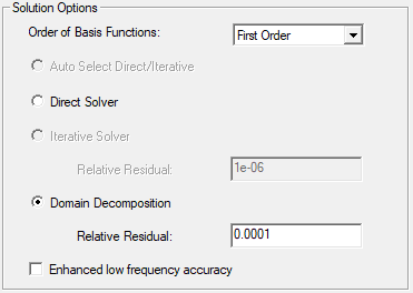

The domains are UI defined through the array definition, not solver defined domains. Given a valid configuration, an Array solve can use a distributed memory solution.

The UI will provide the antenna array definition to the domain manager. This will cause the following to occur:

1. Instantiation of domains to represent the cells of the antenna array plus surrounding air padding cells.
2. Creation of internal domain manager data structures that are needed to support the solve and post processing. This includes appropriate domain parent/child relationships, transformations from the physical domain, interface information per pair of domains, and support for locating a domain by row/column coordinates within the antenna array.

For linking to the Desktop, the network data from HFSS will include both physical and virtual cells. This applies to both port locations and push excitations.

For Optimetrics solution quantities of both virtual and physical cells can be used for calculation.

For 2D Reports for models with Arrays, matrix solution quantities of virtual cells will be expanded into a vector in the same fashion as without the array. The entries are listed according to their [row, column] order in the corresponding "expanded" matrix.

For Port Field Display there is no GUI change. Only physical ports/terminals will be listed. There is no need to support visualization of user-selected cell (like field overlay plot) because the field patterns of the virtual modes are the same as those in the physical cells.

For designs with an Array, the Edit Sources dialog listing order will be as follows: Sources will be listed according to their cell [row, column] order in the array. For each cell, port/terminals are listed in creation/assignment order with mode in each port listed sequentially. Other type of sources, such as incident waves and linked field sources, will be listed after ports/terminals. You can also create Source Groups for dealing with finite array sources.

There will be no change in the far/near field pattern setup and far/near fields will be computed from radiation surfaces on all cells (both physical and virtual).

Copy/Paste design will copy an array. Copy/Paste geometry will NOT copy an array.

Note: A legacy regular array, with one component with at least two pairs of lattice boundaries, can be opened, but you cannot create a new regular array based on this condition. Regular array can only be created based on native geometries. If you delete a legacy with these conditions, you could only recreate it as a 3D component array.