Setting Up Multi-Objective Genetic Algorithm Optimizer

Setting Up Multi-Objective Genetic Algorithm (Random Search) Optimizer

Follow this procedure to set up an optimization analysis using the Multi-Objective Genetic Algorithm (Random Search) Optimizer. Once you have created a setup, you can Copy and Paste it, then make changes to the copy, rather than redoing the whole process for minor changes.

The Multi-Objective Genetic Algorithm (MOGA) is a hybrid variant of the popular NSGA-II (Non-dominated Sorted Genetic Algorithm-II) based on controlled elitism concepts. It supports all types of input parameters. The Pareto ranking scheme is done by a fast, non-dominated sorting method that is an order of magnitude faster than traditional Pareto ranking methods. The constraint handling uses the same non-dominance principle as the objectives. Therefore, penalty functions and Lagrange multipliers are not needed. This also ensures that the feasible solutions are always ranked higher than the infeasible solutions.

The first Pareto front solutions are archived in a separate sample set internally and are distinct from the evolving sample set. This ensures minimal disruption of Pareto front patterns already available from earlier iterations. You can control the selection pressure (and, consequently, the elitism of the process) to avoid premature convergence by altering the maximum allowable Pareto percentage property.

Set up the variables to optimize in the Design Properties dialog box. The variables must be swept in a Parametric setup.
Click HFSS or Q3D Extractor or 2D Extractor > Optimetrics Analysis > Add Screening & Optimization . The Setup Optimization dialog box appears.

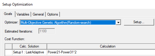
Under the Goals tab, select the optimizer by selecting Multi-Objective Genetic Algorithm (Random Search) from the Optimizer drop-down list.

Optionally click Setup to open the Optimizer Options dialog box.

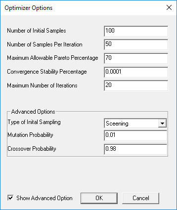
Number of Initial Samples – Initial number of samples to use. This number must be greater than the number of enabled input parameters. The minimum recommended number of initial samples is 10 times the number of enabled input parameters. The larger the initial sample set, the better your chances of finding the input parameter space that contains the best solutions.

The number of enabled input parameters is also the minimum number of samples required to generate the Sensitivities chart. You can enter a minimum of 2 and a maximum of 10000. The default is 100.

If you switch from the Screening method to the MOGA method, MOGA generates a new sample set. For the sake of consistency, enter the same number of initial samples as you used for the Screening method.

Number of Samples Per Iteration – Number of samples to iterate and update with each iteration. This number must be greater than the number of enabled input parameters but less than or equal to the number of initial samples. The default is for a Direct Optimization system.

You can enter a minimum of 2 and a maximum of 10000.

Maximum Allowable Pareto Percentage – Convergence criterion. Percentage value that represents the ratio of the number of desired Pareto points to the number of samples per iteration. When this percentage is reached, the optimization converges. For example, a value of 70 with Number of Samples Per Iteration set to 200 means that the optimization should stop once the resulting front of the MOGA optimization contains at least 140 points. Of course, the optimization stops before that if the maximum number of iterations is reached.

If the Maximum Allowable Pareto Percentage is too low (below 30), the process can converge prematurely. If the value is too high (above 80), the process can converge slowly. The value of this property depends on the number of parameters and the nature of the design space itself. The default is 70. Using a value between 55 and 75 works best for most problems. For more information, see Convergence Criteria in MOGA-Based Multi-Objective Optimization.
Convergence Stability Percentage – Convergence criterion. Percentage value that represents the stability of the population based on its mean and standard deviation. This criterion lets you minimize the number of iterations performed while still reaching the desired level of stability. When the specified percentage is reached, the optimization is converged. The default percentage is 2. To not take the convergence stability into account, set to 0. For more information, see Convergence Criteria in MOGA-Based Multi-Objective Optimization.
Maximum Number of Iterations – Stop criterion. Maximum number of iterations that the algorithm is to execute. If this number is reached without the optimization having reached convergence, iterations stop. This also provides an idea of the maximum possible number of function evaluations needed for the full cycle, as well as the maximum possible time it can take to run the optimization. For example, the absolute maximum number of evaluations is given by:

Number of Initial Samples + Number of Samples Per Iteration * (Maximum Number of Iterations - 1)

Type of Initial Sampling – Advanced option for generating different kinds of sampling. If you do not have any parameter relationships defined, set to Screening (default) or Optimal Space-Filling. If you have parameter relationships defined, the initial sampling must be performed by the constrained sampling algorithms because parameter relationships constrain the sampling. For such cases, this property is set to Constrained Sampling.
Mutation Probability – Advanced option for specifying the probability of applying a mutation on a design configuration. The value must be between 0 and 1. A larger value indicates a more random algorithm. If the value is 1, the algorithm becomes a pure random search. A low probability of mutation (<0.2) is recommended. The default is 0.01. For more information on mutation, see MOGA Steps to Generate a New Population.
Crossover Probability – Advanced option for specifying the probability with which parent solutions are recombined to generate offspring solutions. The value must be between 0 and 1. A smaller value indicates a more stable population and a faster (but less accurate) solution. If the value is 0, the parents are copied directly to the new population. A high probability of crossover (>0.9) is recommended. The default is 0.98.

To Add a cost function, click Setup Calculations to open the Add/Edit Calculation dialog box.

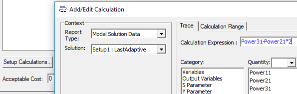
When you have created the calculation, click Add Calculation to add it to the Optimization setup, and Done to close the Add/EditCalculation dialog box.

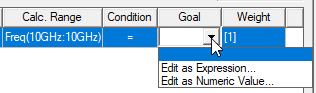
In the Optimization setup, in the Goal column drop-down list, select either Edit as Expression or Edit as Numeric Value.

This reopens the Add/Edit Calculation dialog box. If you are satisfied with the expression or value displayed, click Done to close the dialog box. This enters the expression/value to the Goal column.

In the Optimization setup, if you want to select a Cost Function Norm Type:

Select the Show Advanced Option check box. The Cost Function Norm Type drop-down list appears.

Select L1, L2, or Maximum.

A norm is a function that assigns a positive value to the cost function.

For L1 norm, the actual cost function uses the sum of absolute weighted values of the individual goal errors. For L2 norm (the default), the actual cost function uses the weighted sum of squared values of the individual goal error. For the Maximum norm the cost function uses the maximum among all the weighted goal errors, which means that it is always less than zero. For further details, see Explanation of the L1, L2, and Max Norms in Optimization.

The norm type doesn't impact goal setting that use as condition the "minimize" or "maximize" scenarios.

Optionally, set the Acceptable Cost and Cost Function Noise.
Optionally, click HPC and Analysis Options to select or create an analysis configuration.
In the Variables tab, specify the Min/Max values for variables included in the optimization.

You may also override the variable starting values by selecting the Override check box and entering the desired value in the Starting Value field.
Optionally, modify the values of fixed variables that are not being optimized.
Optionally, set Linear constraints.
Select the View all columns check box to see all columns, including hidden columns.

In the General tab, specify whether Optimetrics should use the results of a previous Parametric analysis or perform one as part of the optimization process.
Select the Update design parameters' value after optimization check box to cause Optimetrics to modify the variable values in the nominal design to match the final values from the optimization analysis.
Under the Options tab, if you want to save the field solution data for every solved design variations in the optimization analysis, select Save Fields And Mesh.
Note:
Do not select this option when requesting a large number of iterations as the data generated will be very large and the system may become slow due to the large I/O requirements.

You may also select Copy geometrically equivalent meshes to reuse the mesh when geometry changes are not required, for example when optimizing on a material property or source excitation. This will provide some speed improvement in the optimization process.