Assigning Finite Conductivity Boundaries

A finite conductivity boundary the behavior of the field at the object surface. The finite conductivity boundary is valid only if the conductor being modeled is a good conductor, that is, if the conductor's thickness is much larger than the skin depth in the given frequency range. If the conductor's thickness is in the range or larger than the skin depth in the given frequency range, HFSS takes the thickness into account, if it has been defined.

To assign a Finite Conductivity boundary:

1. Select a surface on which to assign the boundary and click HFSS>Boundaries>Assign>Finite Conductivity or HFSS>Boundaries>Assign>Surface Roughness>Groiss (Finite Conductivity) ... to bring up the Finite Conductivity Boundary dialog box with Gross selected as the Surface Roughness Model. If you select, HFSS>Boundaries>Assign>Surface Roughness>Huray (Finite Conductivity) ..., the Huray model is selected. For a description of the Huray model, see step 4 below.
   

2. Do one of the following:

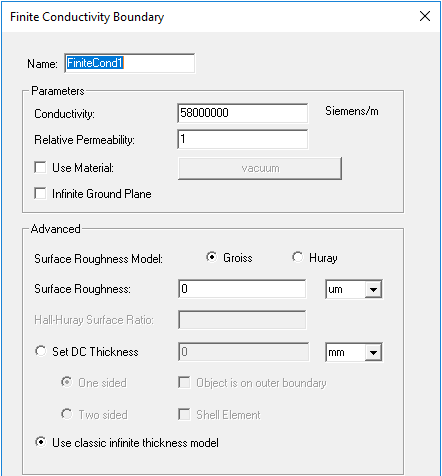
• Enter the conductivity in inverse ohm-meters, and then enter the permeability.

To assign Finite Conductivity so that the boundary is spatially dependent (that is, in which the material properties change over the length), use the method described via this link.

• Select Use Material, click the default material name button , and then choose a material from the material editor. The conductivity and permeability values of the material you select will be used for the boundary. Note that selecting a perfectly conducting material for a finite conductivity boundary triggers a validation error.

3. Select Infinite Ground Plane if you want the surface to represent an electrically large ground plane when the radiated fields are calculated during post processing.

Note that if you select Infinite Ground Plane, the effect of the finite conductivity boundary will be incorporated into the field solution in the usual manner, but the radiated fields will be computed as if the lossy ground plane is perfectly conducting.

For designs with port excitations but no FE-BI boundary and metallic IE region defined, selecting Infinite Ground Plane affects only the calculation of near field and far field radiation during post processing; otherwise, the design has to be re-simulated to model the effects of infinite ground plane. The boundary condition infinite ground plane divides the problem region into two halves. The entire model resides in the half above the boundary, and the radiated fields are set to zero in the half below the boundary. Antenna parameters involving radiated power are consistent with these properties.

Lossy ground planes can be approximated by selecting the Infinite Ground Plane check box when defining Finite Conductivity Boundary or Impedance Boundary. The effects of these boundary conditions are incorporated in the field solution and in the radiated fields accordingly.

Remember the following requirements when defining an infinite ground plane:

• It must be defined on a planar surface.
• All infinite ground planes and symmetry planes must be mutually orthogonal.
• For impedance, layered impedance, or finite conductivity boundaries, only one infinite ground plane can exist in a design. For perfect E boundary conditions, multiple infinite ground planes are supported and they must be co-planar.

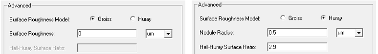
4. Because surface roughness can increase conductor power losses more than two times, HFSS models surface roughness model based on the visible features of copper conductors used in circuit fabrication.To select the Surface Roughness Model used for surfaces such as the interface between the conductor and the substrate for a microstrip line, select either Groiss or Huray.

For the Groiss model, you specify a Surface Roughness parameter (traditional case) as a value (or variable) and units. The default is 0 um. Legacy projects use the Groiss model by default.

For the Huray Model, you specify the Nodule radius value (or a variable), which describes the radius of copper spheres that model the surface roughness. The default is 0.5 um. Also for the Huray model, you specify the Hall-Huray Surface Ratio, a unitless quantity. The default is 2.9. HFSS implements an enhanced version of the Huray surface roughness model. In addition to the benefits of the original Huray model (accurate broad-band modeling of the losses in very rough copper foils typically used in printed circuit board manufacturing), the enhanced model is causal, making it more suitable for time-domain signal integrity studies, and it accurately predicts increased phase delay due to the surface roughness.

(Using surface roughness with the Finite Conductivity boundary may be more intuitive than using a layered impedance boundary to model the effects.)

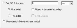
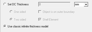
5. You can select either Set DC Thickness or Use classic infinite thickness model. You can specify a DC thickness to more accurately compute DC resistance of a thin conducting object for which Solve Inside is not selected. Skin impedance of the object will be calculated using the defined finite thickness.

To Set DC thickness, click the radio button to enable the Layer Thickness field, and enter a value and select units. You can also specify whether a One-sided object is on outer boundary of the model.

.

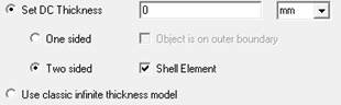
If you select Two sided, you can also specify whether to treat the boundary as a Shell Element. Shell elements maintain two sets of unknown coefficients for the top and bottom surface

Meshing thin layers such as signal traces or thin substrates of PCBs can be difficult and cause very inefficient simulation performance. Instead of meshing these thin layers, they can be replaced with sheets along with appropriately assigned boundary conditions. The appropriate boundaries are 2-sided layered impedance or finite conductivity boundaries where the latter is only applicable for a single layer of metallic material such as a signal trace made of copper.

When to Use Shell Elements

You can consider using shell elements on the sheet for enhanced accuracy at high frequencies where the currents on the two sides of the sheet will be allowed to be different and therefore better model the non-uniform current distribution of a thin structure at high frequencies. Some examples for this application would be studying shielding effects of a car chassis by modeling the chassis with sheets or replacing an antenna radome model with a thin sheet. Note that the shell element option is applicable for all frequencies and can therefore be used for broadband simulations without the need to modify boundary options depending on the simulation frequency. Further, a sheet in the above discussion can also be a face of a solve inside object.

For technical details, see Shell Elements Theory.

The following features are not currently supported when using shell elements:

• Fast sweep
• Scattered field formulation
• Eigen solver
• IE solver

Selecting Use classic infinite model disables the fields for Set DC Thickness and the outer boundary check box.  Calculations for DC then assume infinite thickness.

Also see Assigning DC Thickness under Materials for a discussion of design defaults and the how DC thickness is used and calculated.