
Magnetostatic Field Calculation
In a magnetostatic solution, the magnetic field is produced by DC currents flowing in conductors/coils and by permanent magnets. The electric field is restricted to the objects modeled as real (non-ideal) conductors. The electric field existing inside the conductors as a consequence of the DC current flow is totally decoupled from the magnetic field. Thus, as far as magnetic material properties are concerned, the distribution of the magnetic field is influenced by the spatial distribution of the permeability. There are no time variation effects included in a magnetostatic solution, and objects are considered to be stationary. The energy transformation occurring in connection with a magnetostatic solution is only due to the ohmic losses associated with the currents flowing in real conductors.
The magnetostatic field solution verifies the following two Maxwell's equations:


with the following constitutive (material) relationship being also applicable:

where
-
 is the magnetic field strength.
-
 is the magnetic flux density.
-
 is the conduction current density.
-
 is the permanent magnetization.
-
 is the permeability of vacuum.
- µr is the relative permeability.
For nonlinear materials, the dependency between the H and B fields is nonlinear and can be isotropic or orthotropic (in the case of anisotropic material behavior, µr is a tensor). Similarly, for permanent magnets, nonlinearity can occur in practical cases and is allowed. Additionally, if a demagnetized condition is to be taken into account for (nonlinear) permanent magnets operating below the knee, Maxwell provides an advanced setup option allowing a solution based on a previously computed demagnetization operating point. If nonlinearity occurs in soft materials (with negligible hysteresis) simultaneously with orthotropic behavior, Maxwell requires that the BH curves for the principal directions in the respective material(s) be provided. From these curves, the energy dependency on H is extracted for each of the respective principal directions and is used in the process of obtaining the nonlinear permeability tensor used in the Newton-Raphson iterative solution process:


where  and
and  are the previous field solution,
 is a general full tensor, and [µ] is given by the
following:
is a general full tensor, and [µ] is given by the
following:

with µx, µy, µz taking into account the anisotropic effects of any laminations present in the model.
The 3D magnetostatic solver considers the magnetic field H with the following components:

where j is the magnetic scalar potential,  is a particular
solution constructed by assigning values to all the edges in the mesh
in such a way that Ampere's law holds on all contours of all tetrahedra
faces in the mesh, and
is a particular
solution constructed by assigning values to all the edges in the mesh
in such a way that Ampere's law holds on all contours of all tetrahedra
faces in the mesh, and  accounts for the permanent magnets if any. Thus, the DOFs are
the nodal values of the magnetic scalar potential with ten values per
tetrahedron at each of the four vertices and all six mid-edge nodes,
ensuring a quadratic approximation inside each finite element; i.e. the order of the magnetic scalar potential is 2.
accounts for the permanent magnets if any. Thus, the DOFs are
the nodal values of the magnetic scalar potential with ten values per
tetrahedron at each of the four vertices and all six mid-edge nodes,
ensuring a quadratic approximation inside each finite element; i.e. the order of the magnetic scalar potential is 2.
There are major advantages of this formulation over other existing ones, including using considerably fewer computational resources (due to the scalar nature of the DOFs), not requiring a gauge due to excellent numerical stability, significantly reducing cancellation errors, and capably of automatically multiplying connected iron regions. The magnetostatic solver handles both 3D linear and nonlinear problems. In the case of nonlinear applications, a classic Newton-Raphson iterative algorithm with user-controlled accuracy is used.
The magnetostatic solver calculates the magnetic field distribution produced by a combination of known DC current density vector distribution and a spatial distribution of objects with permanents magnetization. It is also possible to apply boundary conditions to a model such that the simulation of the immersion of a device into an external magnetic field is also possible. In this latter case, the boundary conditions should be applied in such a way that Maxwell's equations are not violated inside the domain of the solution or at the boundaries.
Typical sources for magnetostatic field problems include voltage, current, permanent magnetization, and current density. When applying the sources for the magnetic field problems, the applied current distribution must be divergence free in the entire space of the solution as it is physical for quasi-stationary conduction current density distributions. Thus, the conduction paths(s) for the applied current distributions must be closed when totally contained within the solution space for the problem, or must begin and end at the boundaries.
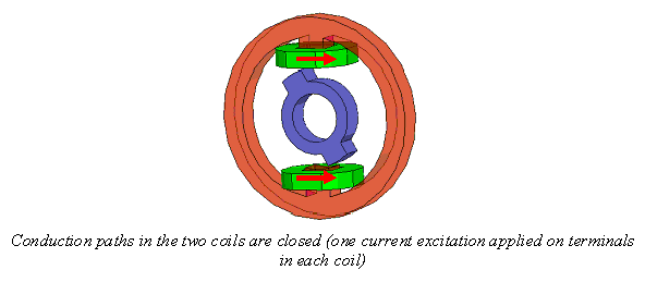
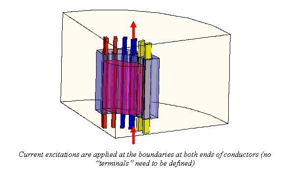
The total current applied to conductors that touch the boundaries does not require the existence of terminals at the ends where the current is applied because the respective planar surfaces of the conductors in the plane of the region (background) can be used to apply the excitations. In the case of a closed conduction path, a terminal (sheet object) must be created, matching the cross-section of the conductor at the desired location such that the excitation (current/voltage) can be applied.
Voltage excitations (at least two) must be specified such that the current can flow in the respective conductors to form an uninterrupted conduction path. Voltage drop excitation should by used in the case of closed conduction paths (possibly containing objects with different electric conductivities), primarily in situations where the total current is unknown. One voltage drop excitation per conduction path should be applied. The total current for any conduction path should add up to zero.
The magnetostatic solver does not compute the electric field distribution associated with a voltage distribution outside conductors. However, the electric field inside conductors is indirectly available for postprocessing via the conduction current density distribution, which is available, so it is possible to calculate the ohmic loss in conductors with applied current or voltage excitations.
Permanent magnetization in Maxwell is treated as a material property, but we mention it here because of its source characteristics:
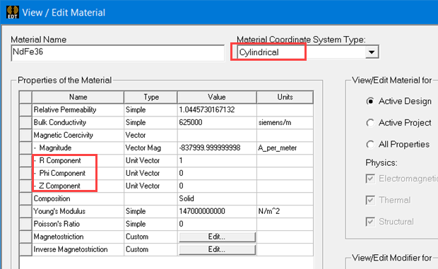
Permanent magnetization can be specified in Cartesian, cylindrical, or spherical material coordinate systems, as shown in the above window where the R, Phi, and Z components (in a cylindrical system, considered here as example) can be specified in any meaningful combination. The actual direction of the vector property is decided when the property is assigned to the object and when the desired coordinate system is chosen (the global coordinate system always exists, while additional ones can be defined). If necessary, additional relative coordinate systems can be defined and used to specify the orientation of the vector property.
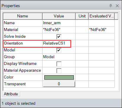
While the type of material coordinate system is embedded into the material definition, the actual orientation is not, such that a material property defined, for instance, in a cylindrical system can be applied to multiple objects with different orientations if multiple relative local coordinate systems were defined and used in the process of assigning the respective material property.
A typical boundary conditions used in magnetostatic problems is the magnetic field tangent (the default, natural boundary condition that is automatically applied on all surfaces of the problem space -the surfaces of the geometry entity containing the model inside it). This default boundary condition can be overwritten if other boundary conditions are applied on exterior surfaces of the solution space. The default boundary condition confines the magnetic field to the solution space; therefore, this boundary must be placed at some distance from the sources to avoid over-constraining the fields by placing the boundaries to close to the model objects. While it is difficult to provide "recipes" with general validity on the placement of the boundaries of problems, a good rule of thumb asserts that if a model can be imagined as being contained in a sphere of radius R, then the boundaries can be placed at a 4-5 radii R from the imaginary center of the model.
The Zero Tangential H Field allows the user to prescribe a normal (in average) field orientation on an arbitrary surface. This boundary condition does not require any further user input, meaning that no value and coordinate system specification are necessary.
In the case of Tangential H Field boundary condition, the values of two tangential components and a surface coordinate system must be defined and subsequently used in the assignment process of this boundary condition. This boundary condition is restricted to two kinds of surfaces: planar or cylindrical. The CS in the planar case would be a rectangular coordinate system with X and Y components of H in the plane. The coordinate system in the cylindrical case would be a coordinate system with a Z axis coinciding with the axis of the cylinder, and the two components to input would be the PHI and Z axis components of H.
In the case of the tangential H field, caution is advised: This boundary condition should be specified such that Ampere's theorem is not violated inside the field domain or at the boundaries.
Symmetry boundary conditions are used to solve problems with symmetry and, thus, allow the users to take advantage of the significantly reduced problem size for a given accuracy.
Symmetry boundary conditions can be one of two kinds:
- Odd (flux tangent)
- Even (Flux normal)
Although the use of this symmetry boundary condition overlaps with previous conditions to some extent, the symmetry boundary conditions should only be used in clear symmetry cases.